

Building a Chess Engine Without Neural Networks
October 25, 2026 · 2 hr 27 min read
Every engine at the top of the computer chess rating lists now evaluates positions with a neural network. Stockfish replaced its hand-written evaluation with NNUE and later deleted the classical code entirely. The hand-crafted evaluation, a list of chess rules with numeric weights, is generally considered an obsolete art.
Heaven’s Gate is a chess engine with no neural network in it. It is about 10,000 lines of C++20: bitboard move generation, a principal variation search with the standard modern selectivity, and an evaluation made of 1,158 integer weights. Measured against engines with published CCRL Blitz ratings, it moved from about 2361 to about 3024 on an anchored scale. You can play against the engine directly in your browser at heavensgateonline.vercel.app.
Before settling on that linear evaluation, the engine began with a design that was neither classical nor neural: an evaluator built on spectral graph theory and tropical algebra.
When modern engines evaluate chess positions with neural networks (whether NNUE or deep convolutional nets), they treat evaluation as high-dimensional statistical curve-fitting. You feed tens of thousands of sparse coordinates or tensor planes into layers of unconstrained weights, letting gradient descent discover arbitrary statistical correlations from millions of self-play games. A spectral-tropical approach comes from a completely different intellectual lineage. Instead of empirical statistical regression, it attempts an analytical, coordinate-free physical theory of the board:
- It treats the pieces as vertices in a continuous, weighted spatial graph, using the combinatorial graph Laplacian () to compute real-valued topological invariants: the Fiedler eigenvalue () for piece coordination, the spectral gap, and Cheeger conductance bottlenecks, treating piece harmony like vibrational frequencies or heat diffusion across a physical circuit.
- Then, instead of mapping those invariants through conventional linear algebra over the real field , it evaluates them over the max-plus semiring of tropical geometry, where addition is maximum and multiplication is addition: the mathematics of shortest paths, dynamic programming, and piecewise-linear polyhedral cones.
It was an attempt at an analytical physics of chess rather than a statistical neural net. The reason that geometric dream failed, and how a transparent linear model succeeded in its place, is one of the central stories of the engine.
What makes it worth writing about
None of the individual techniques in Heaven’s Gate are new; alpha-beta, Texel tuning and SPSA are all decades-old or well documented. What is less common is the combination, and the evidence attached to it:
- It sits in a range few hand-crafted engines reach. An anchored rating near 3000 on the CCRL Blitz scale puts it well into master-engine territory, with an evaluation a person can read line by line and a search that runs on one core. There is no network, no GPU and no opaque weights file: every one of the 1,158 numbers in the evaluation has a name and a meaning.
- The tuner fits the real engine, not a copy of it. Most tuners reimplement the evaluation in a form they can differentiate. This one measures each coefficient by perturbing the engine’s own evaluation function, and refuses to run unless its model reproduces the engine to within centipawns. The weights it produces are exactly optimal for the code that plays, which is a stronger guarantee than tuning usually gives.
- Every claim is tested, including the failures. Every change went through a pentanomial sequential test against the previous version, and the negative results are published here alongside the positive ones: 33 candidates, 8 merged. The rating comes from matches against independently rated engines, not from self-play.
- It learns from its own games. The latest evaluation was refitted on positions harvested from the engine’s own test games, so the data it trains on is concentrated on the positions it actually reaches.
- It is built on a documented failure. The first version did not use an NN or classical heuristics; it evaluated positions through graph spectra and tropical algebra. Rather than quietly deleting it, this writeup analyses exactly why an analytical physical theory of piece coordination could not work where empirical linear and neural models succeed, which turned out to be one of the most useful parts of the project.
This writeup covers the full stack and the mathematics under each layer:
- the theoretical architecture of spectral graphs and tropical minimax geometry,
- the board representation and why magic bitboards are a perfect hash,
- alpha-beta search, its complexity bounds, and the pruning rules that break them,
- the mathematical post-mortem of why the spectral-tropical model broke down under real-time search,
- the linear evaluation that replaced it,
- an exact regression method for fitting 1,158 evaluation weights,
- the sequential statistics of deciding whether an Elo gain is real, and
- stochastic approximation (SPSA) for tuning search parameters that cannot be fitted to static data.
One disclosure up front: the engine contains no network, but the positions its weights were fitted to were labelled by Stockfish, which does. The features are hand-designed; the regression targets came from a stronger engine.
1. The Theory: Spectral Graphs and Tropical Minimax Geometry
Modern chess engines are almost universally built on neural networks. Whether using NNUE (Efficiently Updatable Neural Networks) in Stockfish or deep convolutional and residual networks in Leela Chess Zero, the prevailing methodology frames position evaluation as high-dimensional statistical pattern matching. You project tens of thousands of sparse coordinates or tensor planes into layers of unconstrained weights, allowing gradient descent to extract empirical correlations across millions of self-play games.
A neural network has no built-in notion of geometric space, graph connectivity, or physical force. To an NNUE, a chess position is a high-dimensional binary vector; to a deep convolutional network, it is a stack of spatial bit-planes processed through brute-force tensor contractions.
Heaven’s Gate began from a completely different intellectual lineage: an attempt at an analytical, coordinate-free physics of the board. Rather than fitting millions of opaque weights to game outcomes, the initial engine modeled the chess board as an interconnected dynamical system:
- The Spatial Graph: Every piece on the board is a vertex in a weighted graph, whose edges represent physical lines of force, defense, attack, and multi-piece batteries.
- Spectral Graph Theory: The combinatorial graph Laplacian () acts as a discrete Laplace-Beltrami operator across the board. Its spectral invariants (the Fiedler value , Dirichlet energy, and Cheeger conductance bottlenecks) measure piece coordination and structural vulnerability directly from the spectrum, treating tactical harmony like vibrational modes or diffusion on a network.
- Chebyshev Graph Convolutions: Higher-order multi-hop piece coordination (such as a queen backing a bishop on a long diagonal, or doubled rooks on an open file) is captured without expensive matrix diagonalization via truncated Chebyshev polynomials of the normalized Laplacian ().
- Tropical Minimax Geometry: Instead of passing these invariants into conventional linear algebra or black-box neural layers, the engine evaluated them over the max-plus semiring of tropical geometry: the native algebra of minimax trees. By evaluating positions as dual-surface tropical rational functions () across 10 Spatial King Buckets, the evaluator constructed a piecewise-linear, non-convex polyhedral decision surface.
The Piece Interaction Tensor
A standard bitboard representation records piece locations as 64-bit integers. While optimal for bitwise move generation, it isolates pieces from one another: a knight on f3 is merely a bit in a register, containing no direct information about the pawn it anchors on e5 or the enemy king it pressures on g8.
To capture the board as a physical force network, the engine transforms the position into a dynamic weighted undirected graph . The vertex set consists of all active pieces on the board (, shrinking dynamically as pieces are captured). The edges represent tactical and spatial interactions, quantified by a symmetric adjacency matrix .
The edge weights are defined by a piece-interaction tensor scaled by spatial distance:
For any two pieces on square and on square :
- Direct Defense (Same Color): Base weight (e.g. a pawn defending an outpost knight).
- Direct Attack (Opposing Colors): Base weight (e.g. a bishop striking an enemy queen).
- Ray Battery / X-Ray Support: When two pieces share a rank, file, or diagonal with no intervening pieces of lower value, . This explicitly encodes rook batteries along open files and queen-bishop batteries on long diagonals.
- Chebyshev Distance Decay: Tactical influence decays with king-move distance :
The adjacency matrix is zero along the main diagonal () and strictly symmetric ().
The Graph Laplacian and Discrete Dirichlet Energy
From the adjacency matrix , the degree matrix is the diagonal matrix of row sums:
The combinatorial graph Laplacian is defined as:
In continuous physics, the Laplace-Beltrami operator governs diffusion, wave propagation, and electrostatic potential. On the discrete piece graph, acts as its discrete analogue. For any signal vector assigning a potential value to each piece , the quadratic form computes the discrete Dirichlet energy across the network:
Because , this sum of squares is non-negative for all . Hence is symmetric positive-semidefinite (), and all its eigenvalues are real and non-negative:
The smallest eigenvalue corresponds to the trivial uniform eigenvector , since .
Algebraic Connectivity () and the Cheeger Bottleneck
The second smallest eigenvalue, , was introduced by Miroslav Fiedler in 1973 and is known as the Fiedler value or algebraic connectivity. By the Courant-Fischer Rayleigh-Ritz theorem, it satisfies:
In physical systems, measures how easily energy diffuses through a medium; in structural mechanics, it measures the stiffness of a truss. In Heaven’s Gate’s theoretical formulation, served as a scale-invariant measure of piece coordination:
- High Algebraic Connectivity (): The player’s pieces form a cohesive, mutually defending web. Rooks connect along ranks, minor pieces anchor central outposts, and the structure is resilient to tactical disruptions.
- Low Algebraic Connectivity (): The piece network is fragmented into isolated clusters. A stranded queen on the rim or an undeveloped rook produces a near-zero Fiedler value, signaling vulnerability to forks and deflection tactics.
The mathematical bridge from the spectrum to tactical weakness is the Cheeger inequality. For a graph with maximum degree , the Cheeger conductance constant measures the worst-case structural bottleneck:
Cheeger’s inequality bounds this conductance directly by the Fiedler value:
A small Fiedler value proves the existence of a severe topological bottleneck where an opponent can sever defending pieces from the king’s sector.
Multi-Scale Topology: 4 Spatial Subgraphs and Chebyshev Convolutions
A single global Fiedler value averages the entire board into one scalar, which risks washing out localized imbalances (such as a crushing attack on the kingside paired with passive pieces on the queenside). To retain spatial sensitivity, the engine decomposed the piece graph into 4 Localized Spatial Subgraphs:
- Kingside Zone (): Files f, g, h. Measures kingside attacking momentum and castled shield stability.
- Queenside Zone (): Files a, b, c. Measures flank pawn storms and queenside file control.
- Center Zone (): Files d, e. Measures central space occupation and piece transit.
- Back-Rank Zone (): Ranks 1-2 for White, ranks 7-8 for Black. Measures back-rank vulnerability and piece development.
By extracting per-side Fiedler values and across each zone, the model generated 8 localized spectral invariants.
Furthermore, tactical chess combinations rely on multi-hop indirect coordination: a queen aligned behind a bishop on a long diagonal, or doubled rooks along an open file. In graph signal processing, spectral convolutions filter signals across graph topologies:
where is the complete Laplacian eigendecomposition. Computing on every evaluation call is far too slow for tree search. Hammond et al. and Defferrard et al. showed that spectral filters can be truncated using Chebyshev polynomials on the normalized Laplacian :
The 2-hop Chebyshev graph convolution evaluates 2-step indirect coordination:
Because matrix powers of require only sparse matrix-vector multiplications, propagates indirect tactical support across two edges without computing matrix inverses or full eigendecompositions.
Minimax Geometry over the Tropical Semiring
Once spectral and topological features are extracted into a feature vector , the engine must evaluate that vector into a centipawn score.
Standard evaluations use linear dot products . But linear functions cannot model tactical conditional boundaries: a pawn shield is vital when the king is on g1, but irrelevant if the king has castled queenside. Neural networks solve this by cascading matrix multiplications through non-linear activations (like ReLU), but sacrifice geometric interpretability and require heavy memory bandwidth.
Heaven’s Gate grounded its evaluation in tropical geometry. The max-plus semiring is the algebraic system over with:
Under this semiring, a polynomial takes the form:
A tropical polynomial is a piecewise-linear convex function: the upper envelope of a family of affine hyperplanes.
This is not an arbitrary mathematical choice: tropical algebra is the native algebra of minimax search. When an engine searches a game tree, MAX nodes compute (tropical addition), while path accumulation sums costs and bonuses (tropical multiplication). Evaluating a position through a tropical polynomial corresponds algebraically to evaluating competing tactical hypotheses and selecting the dominant sector.
To handle spatial asymmetry across the board, the engine partitioned positions into 10 Spatial King Buckets (based on the enemy king’s location: ranks 1-2 on kingside, queenside, or center; ranks 3-5; ranks 6-8; mirrored for both sides). Each bucket maintained 16 distinct affine sectors:
Dual-Surface Tropical Rational Functions ()
A single tropical polynomial is convex by construction. But chess evaluation is inherently non-convex: positional factors like advancing a pawn storm or sacrificing material rise to an optimum and then drop off sharply.
To break convexity without losing the tropical formulation, Heaven’s Gate formulated evaluation as a tropical rational function: the difference of two tropical polynomials:
Here the two surfaces serve distinct tactical roles:
- (Advantage Surface, 160 sectors across 10 buckets): Models material dominance, active piece coordination, passed pawns, and Fiedler connectivity.
- (Vulnerability Surface, 160 sectors across 10 buckets): Models king exposure, structural bottlenecks, tactical pins, and counter-attack avenues.
Subtracting from yields a general non-convex piecewise-linear surface, capable of modeling sharp local penalties, piece traps, and non-monotonic positional dynamics.
To optimize the parameters via stochastic gradient descent (Adam SGD), the non-differentiable maximum was smoothed using the Log-Sum-Exp operator with temperature :
The partial derivatives recover the softmax distribution over sectors:
allowing gradients to flow into each sector proportional to its competitive dominance.
That was the mathematical vision: an engine whose understanding of the board sprang from continuous topological invariants and tropical minimax geometry rather than unconstrained neural curve-fitting.
To understand why this model ultimately could not survive competitive play, we must first examine how a modern chess engine generates moves (Section 2) and traverses millions of branches per second in search (Section 3). The severe computational and game-theoretic realities that emerge under the clock will then lead directly to our mathematical audit in Section 4.
2. Board Representation
Bitboards
The engine represents a position as twelve 64-bit integers, one per piece type and colour, where bit is set if square (a1 = 0, h8 = 63) holds that piece. Set algebra on squares becomes bitwise arithmetic: the occupancy is , the squares a knight on can move to are , and the number of such squares is a single popcount.
Moves are packed into 16 bits (6 for the origin, 6 for the destination, 4 for the type: quiet, double push, two castles, capture, en passant, and eight promotion kinds), small enough that a transposition-table slot can carry one inside a single 64-bit data word.
class Move { uint16_t data_{0};public: constexpr Move(Square from, Square to, MoveType type = MoveType::Quiet) noexcept : data_(static_cast<uint16_t>(from) | (static_cast<uint16_t>(to) << 6) | (static_cast<uint16_t>(type) << 12)) {} constexpr Square from() const noexcept { return static_cast<Square>(data_ & 0x3F); } constexpr Square to() const noexcept { return static_cast<Square>((data_ >> 6) & 0x3F); }};Sliding attacks as a perfect hash
Knight and king attacks depend only on the square, so they are 64-entry tables. Rook, bishop and queen attacks also depend on the occupancy along their rays. For a rook on square , let be the relevant-occupancy mask: the squares on its rays, excluding the board edge (an edge square never blocks anything beyond itself). The attack set is a function of only bits, at most 12 for a rook and 9 for a bishop.
We want a map from the blocker subsets to table indices that is cheap and collision-free up to equal outputs. The magic construction uses
one 64-bit multiply and one shift. Multiplication by shifts and adds copies of the blocker bits; a good routes each relevant bit into the top positions without destructive carries for any subset. The engine finds each at startup by rejection sampling: draw a sparse random 64-bit integer (an AND of three uniform draws, so about 8 bits set), and accept it if for all subsets ,
The relaxation in that condition matters. Many blocker subsets share an attack set (anything behind the first blocker on a ray is irrelevant), which is why such small perfect hashes exist. The rook tables hold entries and the bishop tables 5,248.
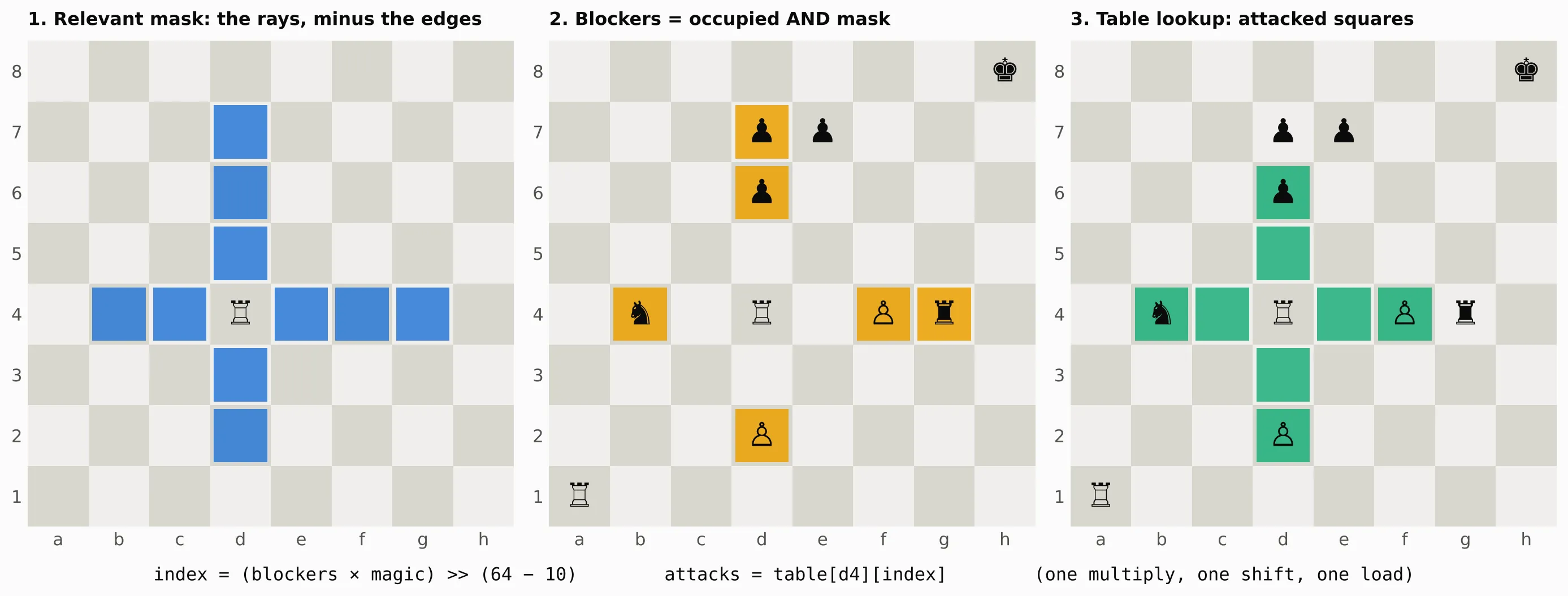 Figure 1: A rook on d4 with relevant squares. (1) The mask . (2) Blockers . (3) The attack set read from the table. It includes our own pieces on f4 and d2; move generation removes them with .
static Bitboard rook_attacks(Square sq, Bitboard occupied) noexcept { const MagicEntry& m = rook_magics_[static_cast<size_t>(sq)]; Bitboard occ = occupied & m.mask; size_t idx = static_cast<size_t>((occ * m.magic) >> m.shift); return m.attacks[idx];}Zobrist hashing
Each position is identified by a 64-bit Zobrist key: an XOR of independent random 64-bit values for every (piece, square) pair present, plus values for side to move, castling rights and the en passant file. Because XOR is its own inverse, a move updates the key in : . With full 64-bit keys stored in the table, a false match between two different positions has probability on the order of per comparison, which is negligible at the roughly probes of a long game.
Correctness by perft
Move generation is verified by perft: the exact count of leaf nodes of the legal-move tree at fixed depth. From the initial position, depth 6 has 119,060,324 leaves. Heaven’s Gate matches the standard perft suite exactly, at 57 to 110 million leaves per second, and every change to the board code is checked against it first.
3. Search
Negamax and the cost of exhaustive search
For a zero-sum game with alternating moves, the value of a position to the side to move satisfies the negamax recurrence
With branching factor , a depth- search visits nodes. Depth 6 is about .
Alpha-beta and the Knuth-Moore bound
Alpha-beta carries a window : is a score the side to move is already guaranteed elsewhere, a score the opponent will not allow. Once a move scores , the node’s remaining moves are irrelevant, since the opponent will avoid reaching it.
def alphabeta(board, depth, alpha, beta): if depth == 0: return evaluate(board) for move in ordered(board.legal_moves()): board.push(move) score = -alphabeta(board, depth - 1, -beta, -alpha) board.pop() if score >= beta: return score # fail high: refutation found alpha = max(alpha, score) return alphaThe result equals the minimax value; only the work changes. Knuth and Moore showed that with perfect move ordering the number of leaves visited is
The argument classifies nodes into three types. At a PV node every child must be searched; at a cut node only the first (best) child is needed to produce a refutation; at an all node every child is searched, but each child is a cut node. Along any path the two non-PV types alternate, so only every second ply branches fully, and the tree behaves like one of depth . The effective branching factor drops from to roughly .
I measured this directly with a material-only evaluation on three middlegame positions:
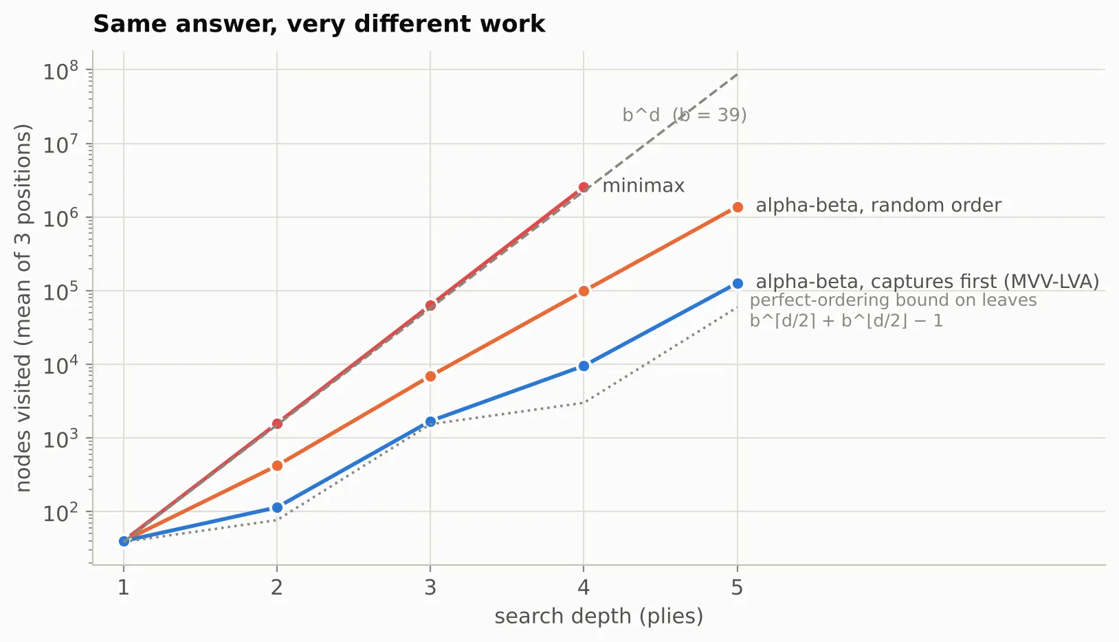 Figure 2: Nodes visited (mean branching factor 39). At depth 4: minimax 2.5 million, alpha-beta with random move order 98,000, alpha-beta trying captures first by MVV-LVA 9,500. The dotted line is the Knuth-Moore bound on leaves.
The gap between random and ordered alpha-beta is a factor of ten at depth 4 and grows with depth. Heaven’s Gate orders moves as: the transposition-table move, winning captures (by static exchange evaluation, then capture history), two killer moves per ply, the countermove to the opponent’s previous move, castling, quiet moves by a weighted sum of history tables
where is butterfly history and is continuation history indexed by the move plies earlier, and finally losing captures.
Static exchange evaluation
SEE estimates the material outcome of a capture sequence on one square without making moves. With the value of the first victim, each recapture by the least valuable attacker gives
and the result is folded back with the option to stop: . X-ray attackers are revealed by removing each capturing piece from the occupancy bitboard and recomputing slider attacks on the target square. The engine uses a thresholded form, see_ge(move, t), which can stop early once the outcome is decided relative to .
Transposition table
The TT caches (best move, score, depth, bound type) per Zobrist key, four 16-byte slots per 64-byte cache line. With several threads sharing it, concurrent writes can tear an entry. The engine uses the Hyatt-Mann XOR scheme instead of locks: store in place of the key . A reader that observes data from one write and from another recovers and treats the slot as a miss.
struct TTSlot { std::atomic<uint64_t> key_xor{0}; std::atomic<uint64_t> data{0}; uint64_t load_key(uint64_t& data_out) const noexcept { data_out = data.load(std::memory_order_relaxed); return key_xor.load(std::memory_order_relaxed) ^ data_out; } void write(uint64_t key, uint64_t new_data) noexcept { data.store(new_data, std::memory_order_relaxed); key_xor.store(key ^ new_data, std::memory_order_relaxed); }};Iterative deepening, PVS and aspiration windows
The engine searches depth until time runs out. Since the tree grows geometrically with ratio , the total cost is dominated by the last iteration, , and earlier iterations pay for themselves by seeding the TT and history tables.
Principal variation search searches the first move with the full window and every later move with a null window , which only decides whether the move beats . A null-window search fails faster because it generates more cutoffs; only moves that fail high are re-searched with the full window. Aspiration windows start each iteration at around the previous score with centipawns and grow by a factor of 1.5 on each failure.
Quiescence search
At the horizon, a static evaluation in the middle of an exchange is meaningless. The quiescence search extends every leaf with captures (and all evasions in check) until the position is quiet, with the stand-pat score as a lower bound, since the side to move may decline to capture:
int stand_pat = in_chk ? -ScoreInfinity : Evaluator::evaluate_fast(board, alpha, beta);if (!in_chk) { if (stand_pat >= beta) return beta; if (stand_pat > alpha) alpha = stand_pat;}for (size_t i = 0; i < moves.size(); ++i) { MovePicker::pick_best(moves, scores, i); const auto& m = moves[i]; if (!in_chk) { // SEE pruning: skip exchanges that lose material. if (!m.is_promotion() && !MoveGenerator::gives_check(board, m) && !MovePicker::see_ge(board, m, 0)) continue; // Delta pruning: even winning the victim for free cannot reach alpha. if (stand_pat + victim_value(m) + 200 < alpha && !m.is_promotion()) continue; } board.make_move(m); int score = -quiescence_search(board, -beta, -alpha, ply + 1); board.unmake_move(m); // ... cutoff and alpha update ...}The stand-pat assumption is false in stalemate (no move to decline into), so the engine checks for a legal move before standing pat.
Selectivity
Even perfectly ordered alpha-beta grows like . Practical engines reach much greater depth by searching most moves to reduced depth or not at all. Each rule below is a bet that a cheaper search predicts the result of a full one.
Null-move pruning rests on the null-move observation: in most positions, having the move is an advantage. If the side to move passes and a reduced search still scores , a real move would very likely do so too:
if (is_non_pv && depth >= 3 && !in_chk && eval >= beta && static_eval >= beta - 20 * depth && board.has_non_pawn_material(us)) { int R = 3 + depth / 4 + std::min(3, (eval - beta) / nmp_margin); if (!improving) R += 1; R = std::clamp(R, 1, depth - 1); board.make_null_move(); int null_score = -negamax_alphabeta(board, depth - 1 - R, ply + 1, -beta, -beta + 1, ...); board.unmake_null_move(); if (null_score >= beta) { if (depth >= 12) { /* verification search, guards against zugzwang */ } else return beta; }}The observation fails in zugzwang, where every move worsens the position; that is common in pawn endings, hence the non-pawn-material condition and the verification search at high depth.
Reverse futility pruning returns early at depth when : the position is so far above that a shallow search is unlikely to drop below it. Futility pruning is the mirror for : at , quiet moves are skipped when . Both margins were set by SPSA (Section 8).
Late move reductions exploit ordering quality. Move (1-indexed) at depth is searched at depth with
clamped to , and re-searched at full depth only if the reduced search beats :
reduction = lmr_table[std::min(depth, 63)][std::min(i + 1, size_t(63))];if (is_quiet) { reduction -= total_hist / 8192; if (!improving) reduction += 1; if (tt_move && tt_move.is_capture()) reduction += 1; if (!is_non_pv) reduction = std::max(0, reduction - 1);}reduction = std::clamp(reduction, 0, depth - 2);score = -negamax_alphabeta(board, std::max(1, depth - 1 - reduction), ply + 1, -alpha - 1, -alpha, ...);if (reduction > 0 && score > alpha) score = -negamax_alphabeta(board, depth - 1, ply + 1, -alpha - 1, -alpha, ...);Singular extensions do the opposite. If the TT move has a reliable lower bound and a search of all other moves at depth fails low against , the TT move is singular and is searched one ply deeper (two at PV nodes when it fails low by a wide margin). Check extensions add a ply when the side to move is in check, which keeps forcing sequences inside the horizon.
To quantify selectivity, I disabled null move and LMR through UCI options and measured nodes to complete each iteration on eight positions:
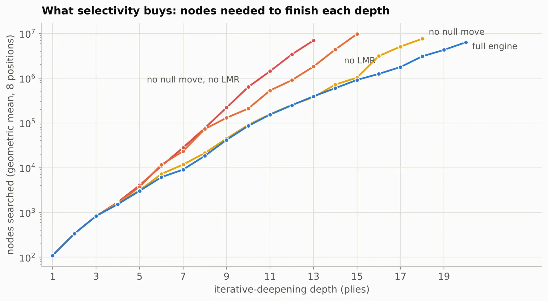 Figure 3: Nodes to complete each depth, geometric mean over 8 positions. The full engine completes depth 13 in about 390,000 nodes and depth 20 in 6.3 million (EBF about 1.5 over the last four plies). Without null move and LMR, depth 13 costs 7.0 million (EBF about 2.4).
Nodes-to-depth is a measure of tree shape, not strength: pruning changes what a given depth means. The only valid measure of a pruning rule is game results.
Time allocation
Between iterations, the engine compares elapsed time to a soft limit, the optimum allocation scaled by three signals:
where decreases with the number of iterations the best move has stayed the same, is the fraction of the iteration’s nodes spent on the best move, and is the score drop from the previous iteration. A stable, dominant best move ends the search early; a falling score extends it. This change alone measured +54 Elo.
4. The Mathematical Post-Mortem: Why the Graph Failed Under the Clock
The physical and geometric theory detailed in Section 1 is mathematically compelling. But a chess evaluation function does not run on paper: it runs under an alpha-beta search traversing millions of nodes per second, where evaluation errors compound exponentially down the tree.
When the spectral-tropical pipeline was tested in real search, every layer of its mathematical apparatus broke down under the clock. It is worth dissecting the exact reasons, both because the breakdown is mathematically instructive and because it explains why classical linear models and neural networks succeed where continuous physics fails.
Why the Spectral Invariants Collapsed
The theoretical appeal of the combinatorial Laplacian was that its spectrum, and specifically the Fiedler value , would measure tactical coordination through the Cheeger conductance bound . In competitive practice, this theoretical connection dissolved:
The graph is complete, so connectivity carries no information. Every pair of pieces has a positive edge, determined only by distance and piece type. It is not an attack graph: a rook behind its own pawn and a rook on an open file get the same weights. A complete graph with positive weights is always connected, so in every position, and its magnitude mostly reflects how spread out the pieces are. On the four test positions I checked, ranged from 5.1 (a sparse endgame) to 14.1 (a crowded middlegame), tracking piece count and density far more than anything resembling coordination.
The trace is a sum of pairwise terms. Since , the “total pressure” feature is a fixed function of piece pairs and their distance, which a hand-crafted evaluation would express directly as a king-tropism or piece-pair table, at a fraction of the cost and with tunable weights per pair.
The eigenvalue estimates were not converged. A chess search cannot afford an QR decomposition per node. To meet time budgets, the engine estimated with four steps of power iteration, then with five steps of power iteration on the shifted matrix after projecting out . Power iteration converges like , which for these spectra (clusters of near-equal eigenvalues, Figure 4) is nowhere near converged after four or five steps. Worse, the first iteration starts from , which is exactly the eigenvector of , so in exact arithmetic and the iteration has nothing to amplify; in floating point it escapes only through rounding error. On my test positions, a float32 reimplementation gave against a true 85.8 on one position, and against a true 11.8 on the same position.
The edge weights depend on vertex order. The opposing-colour weight uses the value of the second endpoint, , and the code computes each edge once for in square order. Since White’s pieces usually occupy lower squares, a White-Black pair is weighted by the Black piece’s value regardless of which piece is attacking, which breaks the colour symmetry an evaluation must have.
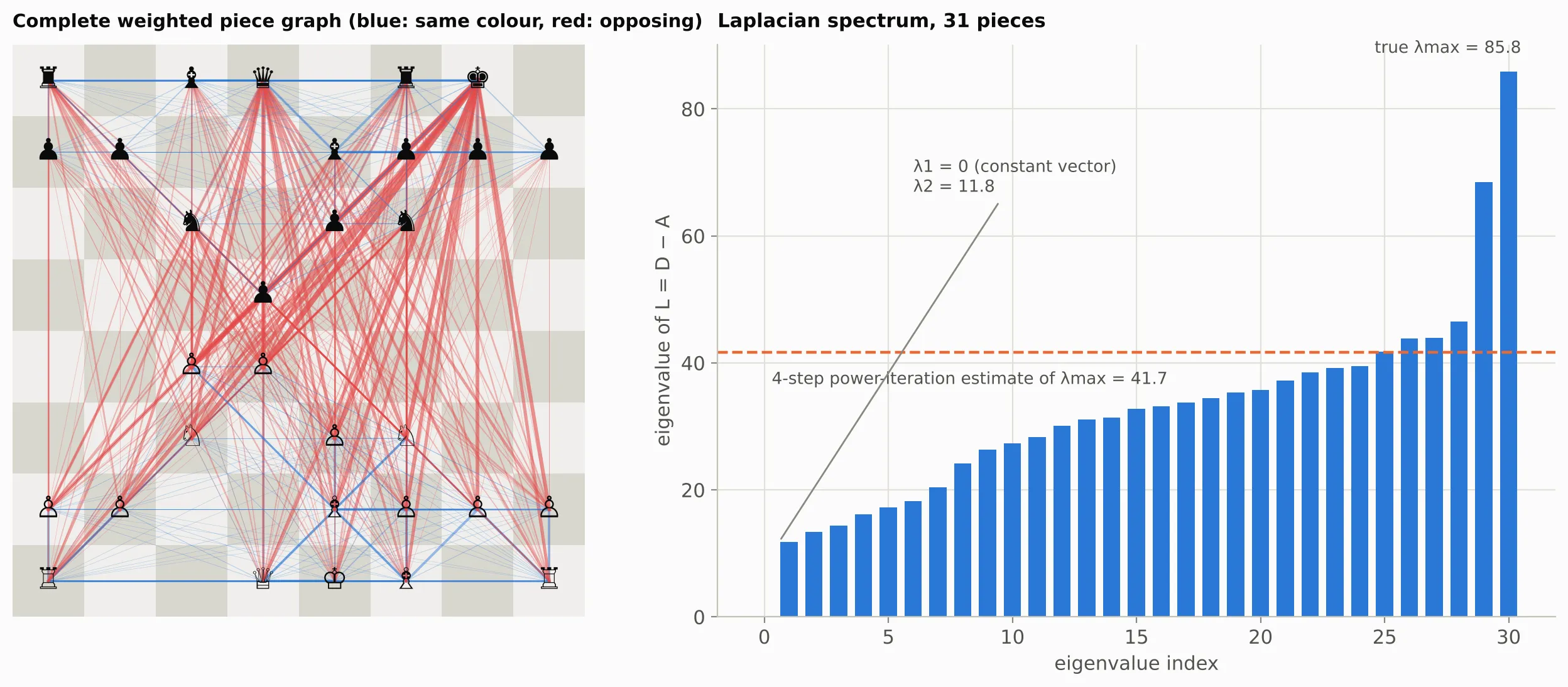 Figure 4: Left: the complete weighted graph of a middlegame position (edge width proportional to ). Right: its exact Laplacian spectrum, computed in double precision, against the engine’s iterative estimate of (from a float32 reimplementation of the same iteration).
Why the Tropical Surface Failed in Search
Evaluating the feature vector through a tropical polynomial or rational function introduced mathematical pathologies of its own:
Convexity cannot capture positional peaks. A maximum of affine hyperplanes is strictly convex, and so is log-sum-exp. Along any feature ray, the evaluation can only bend upward. But chess positional value frequently rises and then falls: the value of advancing pawns in a storm, of king activity versus exposure, or of piece mobility versus defensive duty. A convex model cannot represent an interior optimum in any direction.
Softmax smoothing adds a position-dependent bias. Writing , the bounds give, after taking :
With internal units, and the output scaled by 10 into centipawns, the gap is up to centipawns. Where in that 125-centipawn window the score lands depends on how many sectors happen to cluster near the maximum, injecting artificial score swings into alpha-beta search windows that have nothing to do with chess.
Dead sectors and vanishing gradients. Under the hard maximum , gradient descent updates only the single winning sector. Any sector that fails to achieve a maximum on early training batches receives zero gradient, permanently freezing its weights. In practice, a handful of sectors monopolized the entire surface while the remaining sectors went dead.
The Contrast: Analytical Physics vs Neural Curve-Fitting
It is instructive to contrast why this analytical architecture collapsed while neural networks like NNUE excel:
- Representation level: NNUE feeds tens of thousands of sparse binary features (half-KP coordinates: piece type, piece square, and king square) directly into wide linear layers, preserving every granular tactical interaction (such as an exact pin, fork, or battery). The spectral-tropical evaluator did the opposite: it aggressively compressed the entire 32-piece board down to 22 scalar invariants (mostly Laplacian eigenvalues and aggregate graph traces), throwing away fine-grained tactical locality under the assumption that global algebraic connectivity was a sufficient summary.
- Geometric structure: Neural networks in chess use unconstrained, highly overparameterized linear combinations whose non-linearities can partition the feature space into millions of complex, non-convex decision regions. The tropical polynomial forced the entire evaluation into a single, globally convex polyhedral cone, where scores could only accelerate upward along extremal rays.
- Optimization mechanics: While modern neural networks benefit from smooth gradient descent across dense parameter spaces with billions of training positions, the hard max-plus surface created dead sectors where gradients vanished for any sector that failed to win, while the iterative eigensolver in front of it injected noisy, unconverged gradients into the backward pass.
What happened to it
The audit that started the strength work found that the spectral-tropical evaluator was not reachable from the playing search in any mode, and its weights file was not in the repository. Every Elo point the engine had came from the classical code path, which is the subject of the rest of this writeup.
5. The Linear Evaluation
The evaluation that plays is a sum of hand-designed terms: material, piece-square tables, pawn structure (doubled, isolated, backward, connected, phalanx, passed pawns by rank with blocker, free-path and king-distance terms), mobility, king safety (shield, storms, open files, weighted king-zone attackers, safe checks), threats, outposts, rook placement, bishop pair, material imbalance and endgame scaling.
Tapered evaluation
Every term has a middlegame weight and an endgame weight. With game phase computed from remaining material (minor 1, rook 2, queen 4), the score is
where scales the endgame component for configurations that are drawish whatever the material count says: opposite-coloured bishops ( or ), two knights against a bare king (), a minor piece up without pawns ( or ).
int Evaluator::evaluate_fast(const Board& board, int alpha, int beta) { const int phase = std::min(24, board.game_phase()); const int tempo = (g_eval_params.tempo_mg * phase + g_eval_params.tempo_eg * (24 - phase)) / 24;
// Lazy cutoff: incrementally maintained material + PST far outside the window. const int simple = /* tapered material + PST, side-relative */; if (simple >= beta + 320 || simple <= alpha - 320) return simple;
const ScorePair w = side_totals(board, Color::White), b = side_totals(board, Color::Black); const int mg = w.mg - b.mg, eg = w.eg - b.eg; const int scaled_eg = eg * eg_scale(board, eg) / 64; const int white_score = (mg * phase + scaled_eg * (24 - phase)) / 24; return (board.side_to_move() == Color::White) ? white_score + tempo : -white_score + tempo;}Material and piece-square sums are updated incrementally in make_move. Pawn terms depend only on the pawn bitboards, so they are cached in a per-thread pawn hash table. The lazy cutoff returns the cheap estimate when it is already decisive relative to the window; removing it cost 35 Elo.
Linearity as a design constraint
Every term is either (count) (weight) or a table entry selected by a count. Mobility, for instance, is a lookup with one weight per number of safe squares:
auto add_mob = [&](PieceType pt, const auto& mg_tab, const auto& eg_tab, auto attack_fn) { for (Bitboard pieces = board.pieces(make_piece(side, pt)); pieces;) { Square psq = pop_lsb(pieces); const size_t count = std::min<size_t>(popcount(attack_fn(psq, occ) & safe_mask), mg_tab.size() - 1); score.mg += mg_tab[count]; score.eg += eg_tab[count]; }};A table is a one-hot encoding: it is linear in its parameters while representing an arbitrary function of the count, including the concave shapes the tropical model could not express. The whole evaluation is therefore linear in its parameter vector , before tapering:
with integer coefficients and residuals for fixed constants. This property is what makes exact fitting possible.
6. Fitting 1,158 Weights
The Texel objective
Texel tuning, introduced by Peter Österlund for his engine Texel, treats the evaluation as a predictor of the expected game score through a logistic link,
and minimises the mean squared error against targets :
is fitted first, by ternary search on the starting weights, and then held fixed; for the current data .
An exact linear model by finite differences
The usual failure mode of a tuner is a reimplementation of the evaluation that drifts from the engine’s. Heaven’s Gate’s tuner never reimplements anything. Since the evaluation is linear in , each coefficient is a finite difference that can be measured by calling the engine’s own evaluation function:
computed separately for the middlegame and endgame components, before tapering:
const ScorePair base = white_terms(b); // the engine's real positional termsfor (size_t j = fd_begin; j < params.size(); ++j) { int* ptr = params[j].engine_ptr; // points into the live eval parameters *ptr += 1; const ScorePair bumped = white_terms(b); *ptr -= 1; const int cm = bumped.mg - base.mg, ce = bumped.eg - base.eg; if (cm || ce) { acc[j].first += cm; acc[j].second += ce; }}Material, piece-square and tempo coefficients come directly from piece placement. The result is a sparse design matrix: 99 million nonzero coefficients over 1.56 million positions, about 64 per position. A --parity mode asserts that the model reproduces the engine’s evaluation to within centipawns, both at the current weights and after random integer perturbations of them, which verifies linearity itself. Adding a non-linear term makes parity fail and the tuner refuse to run.
With and , the gradient is
and the tuner runs full-batch Adam (, , step 0.5) over the sparse matrix, keeping the weights with the lowest validation error.
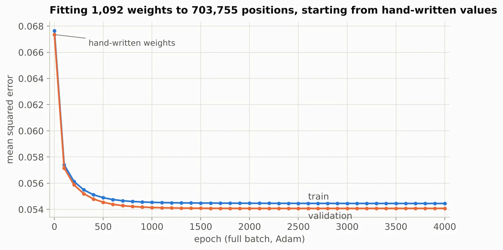 Figure 5: The first fit, of 1,092 weights on 703,755 quiet positions labelled with game results, from hand-written starting values. Validation MSE fell from 0.0674 to 0.0541. That build won its first test by +218 Elo over 160 games, the largest single gain in the engine’s history.
What the fit learned
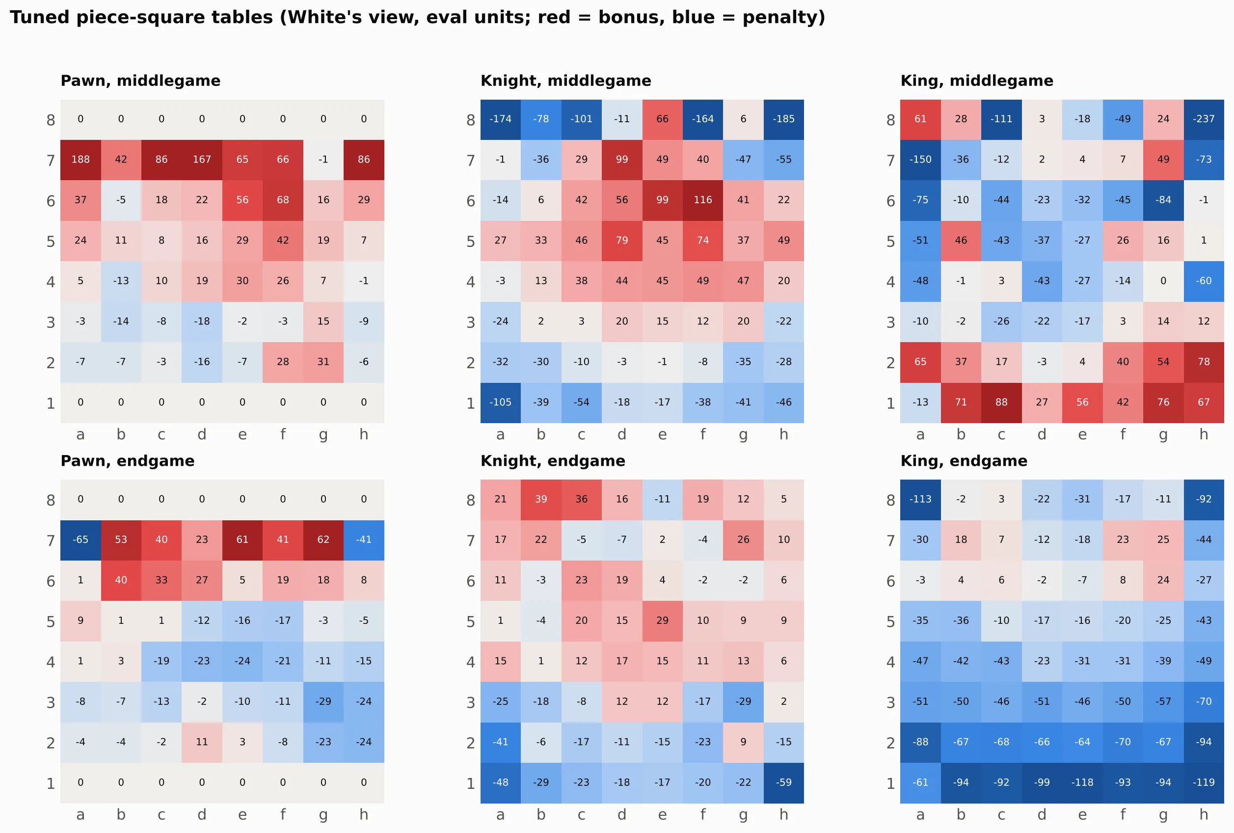 Figure 6: Tuned piece-square tables. Knights favour advanced central squares (f6 +116, e6 +99 in the middlegame) and avoid the rim; the middlegame king prefers b1, c1 and g1.
Two properties of the fitted tables matter for interpretation. Rarely observed squares are poorly constrained (a knight on h8 at -185 reflects almost no data, not chess knowledge). And the tables are not identifiable in isolation: features are correlated, so the endgame king table can be negative near its own back rank because king-distance terms elsewhere already reward activity. Only the sum is meaningful.
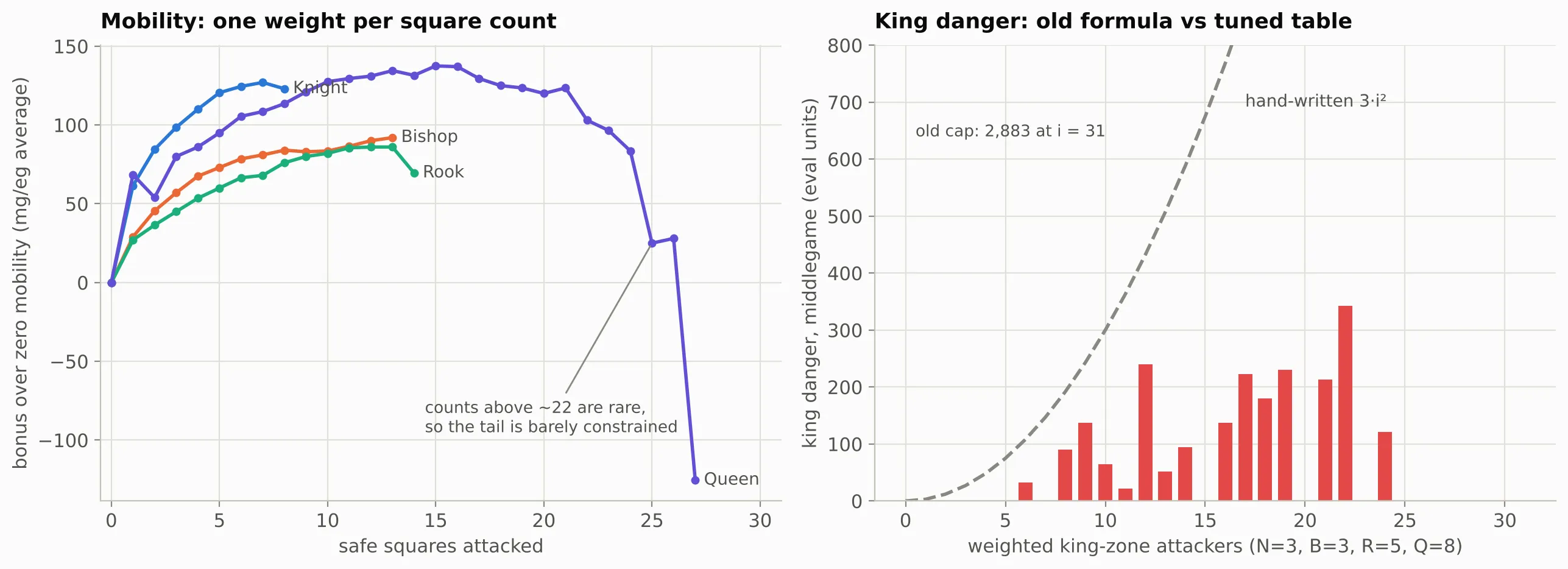 Figure 7: Left: fitted mobility tables, strongly concave in the number of safe squares. Right: the previous hand-written king-danger formula in weighted attackers (one queen near the king cost 192 centipawns; the cap was 2,883) against the fitted table, which stays below 350 and is zero for attacker sums that rarely occur.
Validation loss is not strength
Two later batches of terms (space, pawn islands, king-pawn distance, connected passers, long diagonals, a tunable imbalance, minor pieces behind pawns, king threats and others) each lowered validation error and gained nothing: -14 and 0 Elo over 240 games. Game-result labels are a high-variance target. A position from a game White eventually lost may have been winning for White, so the label noise is of the same order as the signal, and additional features fit the noise. Self-play labels were worse: 1.9 million positions from fast self-play cost 31 Elo, and the fit pulled the rook’s endgame value from 717 to 560, because fast games fail to convert won endgames.
The fix was a better target. Positions were relabelled with Stockfish’s score at 5,000 to 20,000 nodes, blended with the game result,
keeping only quiet positions (best move not a capture, ). With identical features, this gained +50 Elo, material values came out sensible (rook 676/680, queen 1494/1030 in mg/eg), and validation MSE fell to about 0.020, on a different scale because the target variance is much lower. The current fit adds 635,620 positions harvested from about 10,700 of the engine’s own games, for 1.56 million positions in total, which concentrates the data on positions the engine actually reaches.
7. Measuring Real Progress
Why measurement comes first
The early versions of the project reported ratings of “2800” and “3400”. An audit replayed every game in the repository and found that these did not survive scrutiny: the “3400” came from seven games ended early by a mate-score adjudication, with +800 assigned to a perfect score, and the opponents were Stockfish with its strength limiter, which is a handicap target rather than an independent anchor. The first anchored measurement, 400 games against four Blunder releases with published CCRL Blitz ratings at 10+0.1 with every opening played from both sides, gave 2361.
Elo and the pentanomial model
For a score fraction , the logistic Elo difference is
so near equality one percentage point of score is about 7 Elo. Useful changes to a mature engine are worth +5 to +20 Elo, a shift of one to three points.
Every opening is played twice with colours reversed, and the two games are strongly correlated through the opening’s bias. The harness therefore treats each pair as one observation with five outcomes, (the pentanomial model), and estimates
Pairing removes the opening variance from the estimate; treating the games as independent would overstate the precision.
The sequential test
The harness runs a sequential probability ratio test in the normal approximation used by Stockfish’s Fishtest. In normalized Elo, hypotheses and map to pair means with . For Gaussian observations with common variance, the log-likelihood ratio after pairs reduces to
and the test stops when leaves for error rates :
def stats(p): # p = pair-score counts for [0, .25, .5, .75, 1] n = sum(p); xs = [0, .25, .5, .75, 1] mu = sum(x * c for x, c in zip(xs, p)) / n var = sum(c * (x - mu) ** 2 for x, c in zip(xs, p)) / n sg = math.sqrt(2 * var) # per-game std implied by the pair variance mu0, mu1 = 0.5 + elo0 / K * sg, 0.5 + elo1 / K * sg # K = 800 / ln 10 llr = n * (mu1 - mu0) * (2 * mu - mu0 - mu1) / (2 * var) return n, mu, var, llrAll tests used fastchess at 8 s + 0.08 s per move, one thread, 16 MB hash, the UHO_4060_v4 book with both colours per opening, no adjudication, in restart-safe chunks of 40 games. The merge rule was stricter than the SPRT: the 95% confidence interval had to lie entirely above zero.
Resolution and the stacking argument
At these settings, 240 games give a 95% half-width of about 30 Elo. Since the standard error scales as , resolving an effect of size needs roughly
about 1,500 games for . When two independent changes have effects of the same sign, testing them together needs , a factor of about 4 fewer games than either alone. Stacking two well-motivated near-misses resolved twice in this project:
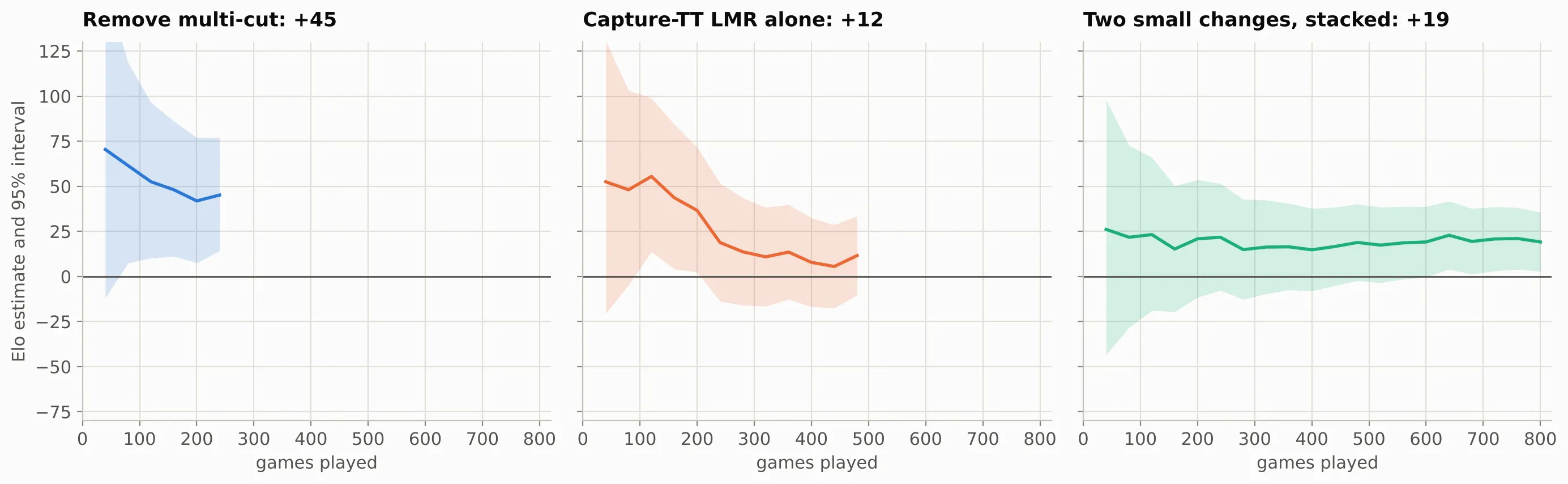 Figure 8: Running estimate with 95% interval. Left: removing classic multi-cut cleared zero within 80 games, ending at +45 [+14, +77]. Middle: one LMR change alone stayed unresolved at +12 [-10, +34] after 480 games. Right: the same change stacked with a null-move condition resolved at +19 [+3, +36] over 800 games.
Results
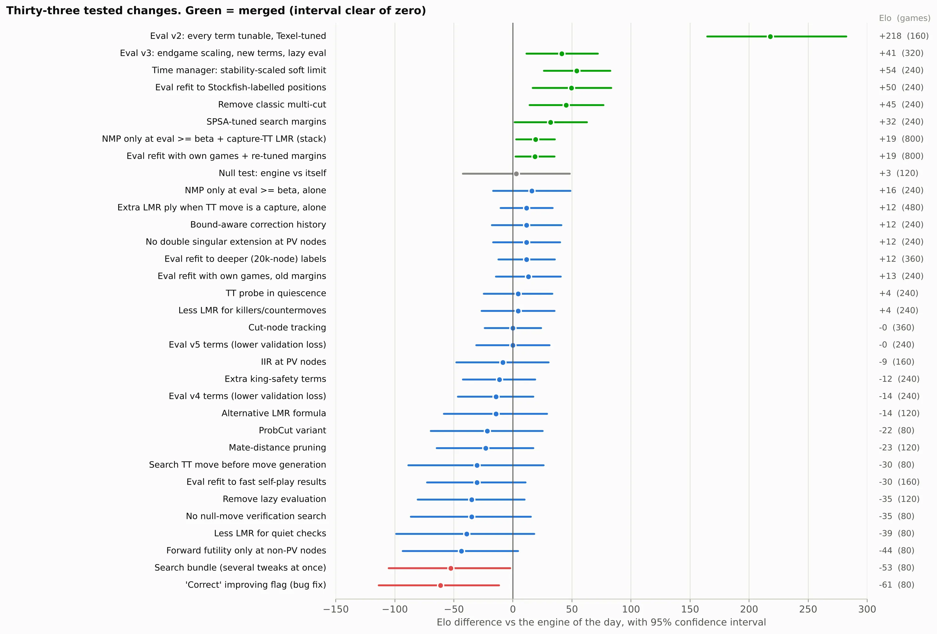 Figure 9: Thirty-three candidates, each against the engine of its day; eight merged. The null test (the engine against itself) measured +3, as a fair harness should.
Several regularities stand out:
- Most changes are neutral or harmful. Techniques standard in strong engines (mate-distance pruning, TT probes in quiescence, IIR at PV nodes, cut-node tracking) did not transfer. A heuristic’s value depends on the rest of the search.
- Correctness and strength are different properties. The
improvingflag compared the static evaluation with a stale value from a sibling node. Fixing it cost 61 Elo, because every pruning margin had been tuned against the buggy flag; the corrected flag pruned less and the search used 33% more nodes per depth. - Bundled changes are uninterpretable. A bundle of search tweaks lost 53 Elo with no way to attribute the loss.
- Deletion is a valid change. The largest search gain, +45, removed a multi-cut pass that duplicated work already done by singular extensions.
Tests run on two cores at fast time controls are sensitive to background load. One test, run while a forgotten SPSA job shared the CPU, lost 31 of 120 games on time and was discarded. Every test PGN is now checked for time forfeits before its result is used; all merged results had none.
8. Tuning the Search with SPSA
Search margins affect play only through the tree, so they cannot be fitted to labelled positions. They were tuned with simultaneous perturbation stochastic approximation. Let be expected match score. Each iteration draws uniformly and plays a short match between and . Since , a Taylor expansion gives
so the match result times is an unbiased (up to ) estimate of the gradient direction from a single match, whatever the dimension . The update is
for k in range(k0 + 1, k0 + 1 + ITERS): delta = {n: random.choice((-1, 1)) for n in names} plus = {n: theta[n] + P[n][1] * delta[n] for n in names} minus = {n: theta[n] - P[n][1] * delta[n] for n in names} W, L = play(plus, minus, games=8, tc="5+0.05") # paired openings, colours reversed r_k = R0 / (1 + k / 400) ** 0.3 for n in names: theta[n] = clamp(theta[n] + r_k * P[n][1] * (W - L) * delta[n])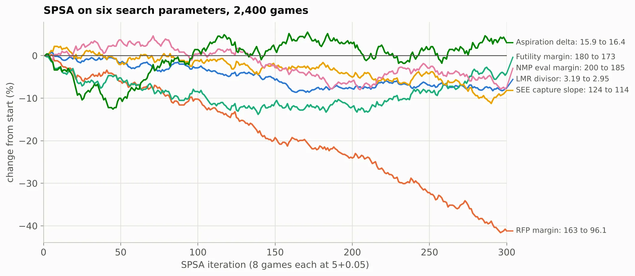 Figure 10: 300 iterations (2,400 games) over six parameters. The reverse futility margin moved from 163 to 96 per ply; the rest changed by 10% or less. Result: +32 Elo [+2, +63].
Evaluation and search parameters are coupled. Pruning margins are thresholds on the evaluation’s scale, and a refit changes both the scale and the balance between terms. When the evaluation was refitted on the engine’s own games, the refit alone measured +13 [-14, +40]. After a second SPSA run on the margins for the new evaluation (reverse futility moved again, from 96 to 70), the pair measured +19 [+2, +35] over 800 games.
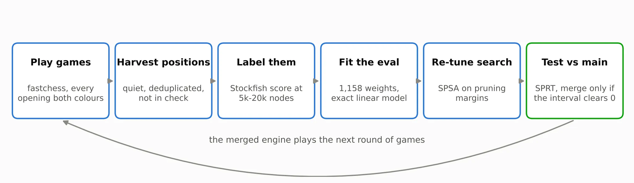 Figure 11: The improvement loop. Games become training positions, Stockfish labels them, the tuner refits the evaluation, SPSA refits the search margins, and the candidate must pass the sequential test against the current version.
9. Results and Limitations
Self-play results measure progress relative to a previous version, not absolute strength. Absolute strength was measured with fixed anchors: Blunder 7.6 (CCRL Blitz 2631) at 10+0.1, and Stockfish with UCI_Elo 2800, 3000 and 3190 at 60+0.6, the control at which its limiter is calibrated. A pooled maximum-likelihood fit over all anchor games gives the rating:
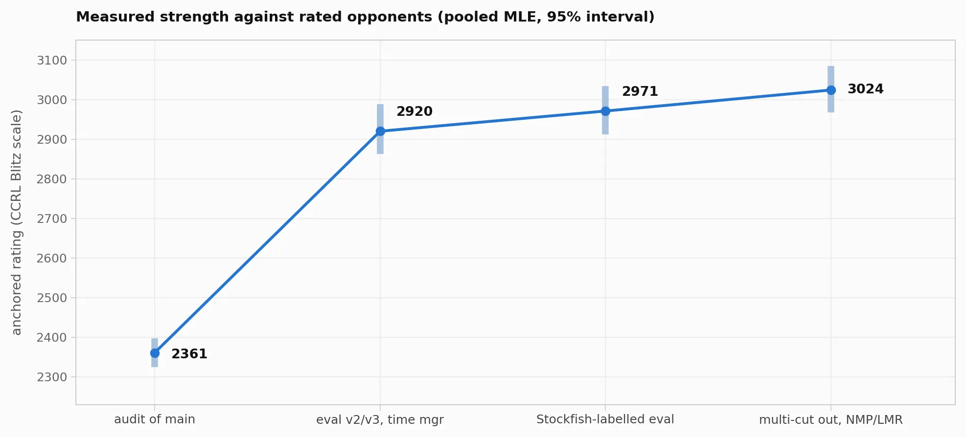 Figure 12: Anchored ratings with 95% intervals at each stage. The latest measured build scored 91% against Blunder 7.6 and 48.8% against Stockfish at 3000, pooling to 3024 (2967 to 3084), with no time forfeits in 220 games.
Two changes merged after that measurement (+32 and +19 in self-play) suggest the current build is somewhat higher; self-play gains usually shrink against other opponents, so no number is claimed until the next anchor match. A check at 2+1 of the engine before and after two merges measured +108 over 40 games, so the fast-control gains carry over to slower play. The anchors were measured on local hardware rather than by CCRL, which adds perhaps 50 to 100 Elo of systematic uncertainty to the absolute figure; the relative progress, 2361 to 3024 under identical conditions, is the robust result.
Error analysis
Every loss against the anchors was analysed with Stockfish, flagging moves that reduced Heaven’s Gate’s win probability by at least 20 points. Of 43 such mistakes, only 9 were missed tactics; the rest were quiet positional misjudgments, mostly in heavy middlegames.
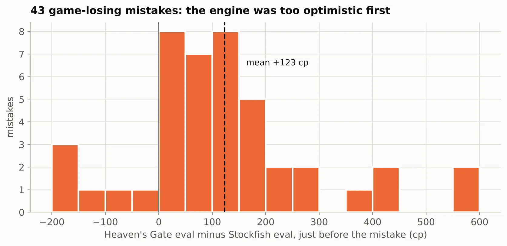 Figure 13: Heaven’s Gate’s evaluation minus Stockfish’s immediately before each of 43 game-losing mistakes (on an earlier build). The mean bias is +123 centipawns; half exceed one pawn.
The engine does not lose for lack of calculation. It loses by overvaluing positions, chiefly through king safety and piece activity in complex middlegames. This is the central limitation of a linear evaluation: terms combine additively, so an interaction such as “this king is safe unless the knight reaches g5 and the h-file opens” must be written in explicitly as a new feature. A network learns such products from data. A hand-crafted evaluation can only approximate them one feature at a time.
Conclusion
Modern computer chess has converged uniformly on neural networks. Whether through NNUE’s sparse feature layers in Stockfish or deep residual networks in Leela Chess Zero, the prevailing consensus is that chess evaluation is an empirical statistical regression: you feed raw board configurations into millions of unconstrained parameters and let gradient descent learn the patterns from vast oceans of game data.
Heaven’s Gate’s first evaluator was a bid to break away from both standard neural networks and classical heuristic lists. Instead of statistical pattern recognition, it tried to formulate chess evaluation as an analytical physics problem: treating piece coordination as vibrational frequencies and Cheeger conductance on a graph Laplacian, and evaluating strategic advantage as an extremal polyhedral surface over the max-plus semiring of tropical geometry.
That it failed is not a flaw in the underlying mathematics, but a lesson in inductive bias. Chess is fundamentally a game of discrete, brittle, non-convex interactions: a single blocked pawn breaks a diagonal, a single weak square collapses a defense, and positional advantage often rises and then falls. Neural networks succeed because their high-dimensional parameter spaces can absorb those messy, non-linear exceptions through sheer data volume. The spectral-tropical model failed because it attempted to smooth that rugged discrete reality into continuous spectral vibrations and convex polyhedra: a complete graph has no connectivity structure to measure, unconverged power iterations do not estimate eigenvalues, and a convex model cannot express an interior optimum.
When Heaven’s Gate finally crossed 3000 Elo, it did so by taking the opposite lesson: not by retreating into an opaque black-box neural network, and not by chasing exotic geometric abstractions, but by building a clean, transparent linear evaluation where every single one of the 1,158 weights has a concrete meaning, an exact regression fit, and a measurable confidence interval.
A hand-crafted engine, done carefully, is a linear model with about a thousand weights, fitted exactly to millions of labelled positions, running under a search whose margins are tuned by stochastic approximation and whose every change must pass a sequential test.
Most of the measured strength came from the plain parts. The +218 came from fitting weights that already existed, the +54 from allocating time better, and the +45 from deleting code. The common thread is that a number without a confidence interval is not a measurement, and a measurement against your own previous version is not a rating.
What I think is genuinely distinctive about Heaven’s Gate is not any single feature but how much of it can be checked. The evaluation is a readable list of chess ideas with fitted weights, the tuner is provably consistent with the engine it tunes, every merged change has an interval attached, every rejected change is on record, and the rating rests on independently rated opponents. That is a different kind of achievement from raw strength: an engine near 3000 where you can point at any number in it and say where it came from and how much it is worth. In an era where the strongest engines are trained black boxes, a strong engine that is fully explainable seemed worth building, and worth writing up.
The engine is open source at github.com/Weptune/Heavens-Gate, and you can play against it directly in your browser at heavensgateonline.vercel.app.
References
- D. Knuth and R. Moore, “An Analysis of Alpha-Beta Pruning”, Artificial Intelligence 6, 1975
- F. Chung, Spectral Graph Theory, CBMS Regional Conference Series in Mathematics 92, AMS
- L. Zhang, G. Naitzat and L.-H. Lim, “Tropical Geometry of Deep Neural Networks”, ICML 2018
- J. C. Spall, “Multivariate Stochastic Approximation Using a Simultaneous Perturbation Gradient Approximation”, IEEE Transactions on Automatic Control 37, 1992
- Texel’s Tuning Method, Chess Programming Wiki
- Fishtest mathematics, for the GSPRT and pentanomial model
- Stockfish (chess), for the NNUE history
- CCRL testing methodology