Your Deck of Cards Isn't Actually Shuffled

Cover art by @prynmatica :3

In a standard deck of 52 playing cards, the number of possible orderings is $52!$, which is roughly $8.0658 \times 10^{67}$. This number is larger than the number of square meters on the surface of every star in the observable universe. If every human who ever lived shuffled a deck once every second since the Big Bang, humanity would still have witnessed less than an infinitesimal fraction of the possible configurations.

Because that permutation space is so vast, most card players assume that almost any chaotic physical mixing is sufficient to make a deck unpredictable. In casual games, and for decades in commercial casinos, dealers would riffle shuffle a deck three or four times before dealing a hand of blackjack or poker. The reasoning felt intuitive: after four shuffles, every single card has been displaced from its original position, cards from the top and bottom of the deck are thoroughly intertwined, and no adjacent pair from the factory order remains intact.

In 1992, mathematicians Dave Bayer and Persi Diaconis published Trailing the Dovetail Shuffle to its Lair. They proved that this intuition is completely wrong.

After four riffle shuffles, the deck is not random. It is not even partially random in any meaningful statistical sense. The mathematical distance between a four-shuffled deck and genuine randomness is $1.0000$ to four decimal places. You can construct bets based on simple card orders where the house has an enormous negative expectation.

Then, between the fifth, sixth, and seventh shuffles, something unusual happens. The distribution of permutations does not slowly drift toward uniform randomness. Instead, it experiences a sharp mathematical phase transition known as the cutoff phenomenon. At six shuffles, the deck remains heavily biased. At seven shuffles, the bias collapses, and the total variation distance drops to $0.334$.

Here is how the mechanics work.

1. The Gilbert-Shannon-Reeds Model

To analyze a physical shuffle mathematically, we need a realistic model of how humans actually shuffle cards.

A riffle shuffle (or dovetail shuffle) consists of two physical steps:

1. The Cut: The dealer cuts the deck of $n$ cards into two packets of sizes $c$ and $n - c$.
2. The Riffle: The dealer releases the cards from their thumbs so that the two packets interleave into a single combined stack.

In 1955, Edgar Gilbert and Claude Shannon developed a probabilistic model for this process at Bell Labs, which was later independently rediscovered by Jim Reeds in 1981. It is now known as the Gilbert-Shannon-Reeds (GSR) model.

The model rests on two simple assumptions:

Step 1: The Binomial Cut

When a human cuts a deck of $n$ cards in half, they rarely divide it into exactly $n/2$ and $n/2$. Instead, the size of the top packet $c$ follows a binomial distribution with parameters $n$ and $p = 1/2$:

$\mathbb{P}(c) = \frac{1}{2^n} \binom{n}{c}$

For $n = 52$, the average cut size is 26, with standard deviation $\sqrt{52 \times 0.5 \times 0.5} \approx 3.6$ cards. Almost all cuts land between 20 and 32 cards.

Step 2: Proportional Interleaving

Suppose the left hand holds a packet of $A$ cards and the right hand holds a packet of $B$ cards. As the dealer lets cards fall from their thumbs, the probability that the next card drops from the left packet is proportional to the size of that packet:

$\mathbb{P}(\text{next card falls from left}) = \frac{A}{A + B}$

$\mathbb{P}(\text{next card falls from right}) = \frac{B}{A + B}$

If the left hand holds 30 cards and the right hand holds 10 cards, the next card is three times as likely to drop from the left hand. As cards drop, the packet sizes $A$ and $B$ shrink until both reach zero.

This physical assumption has an elegant combinatorial consequence: every one of the $\binom{n}{c}$ possible interleavings of the two packets is equally likely.

To see why, notice that if you trace any specific interleaving path backward from $n$ cards to zero, the denominator product in the probabilities telescopes, canceling out the packet counts and leaving exactly $1 / \binom{n}{c}$. Multiplying this by the cut probability $\binom{n}{c} / 2^n$, the combinatorial term $\binom{n}{c}$ cancels entirely:

$\mathbb{P}(\text{specific interleaving with cut } c) = \frac{1}{2^n} \binom{n}{c} \times \frac{1}{\binom{n}{c}} = \frac{1}{2^n}$

In other words, a GSR riffle shuffle chooses uniformly at random among all $2^n$ possible outcomes of binary assignments to cards.

Diaconis and his collaborators tested this model against slow-motion video footage of professional dealers and amateurs. The physical data matched the Gilbert-Shannon-Reeds distribution with remarkable accuracy.

2. Rising Sequences: The Hidden Invariant

The secret to tracking the GSR shuffle lies in an invariant called a rising sequence.

Number the cards in the deck from $1$ to $n$ in their initial factory order, with 1 on top and $n$ on the bottom. After any number of shuffles, the deck is represented by a permutation $\sigma = (\sigma(1), \sigma(2), \dots, \sigma(n))$.

A rising sequence is a maximal subsequence of cards whose face values increase consecutively by $1$, appearing in left-to-right order in the deck.

Let us illustrate this with a small 6-card deck initially ordered:

$(1, 2, 3, 4, 5, 6)$

Suppose we cut the deck into two packets:

• Left packet: $(1, 2, 3)$
• Right packet: $(4, 5, 6)$

Now we interleave them into a new permutation:

$(1, 4, 2, 5, 3, 6)$

How many rising sequences does this permutation have? Let us trace the consecutive numbers:

• Starting with 1: we find $1$, then $2$, then $3$. These form the sequence $(1, 2, 3)$.
• Starting with the next missing number, 4: we find $4$, then $5$, then $6$. These form the sequence $(4, 5, 6)$.

Every card belongs to exactly one rising sequence. The permutation $(1, 4, 2, 5, 3, 6)$ has exactly 2 rising sequences.

Now consider the fundamental theorem of riffle shuffles:

Lemma (Rising Sequence Bound):
A single riffle shuffle can produce at most $2$ rising sequences.

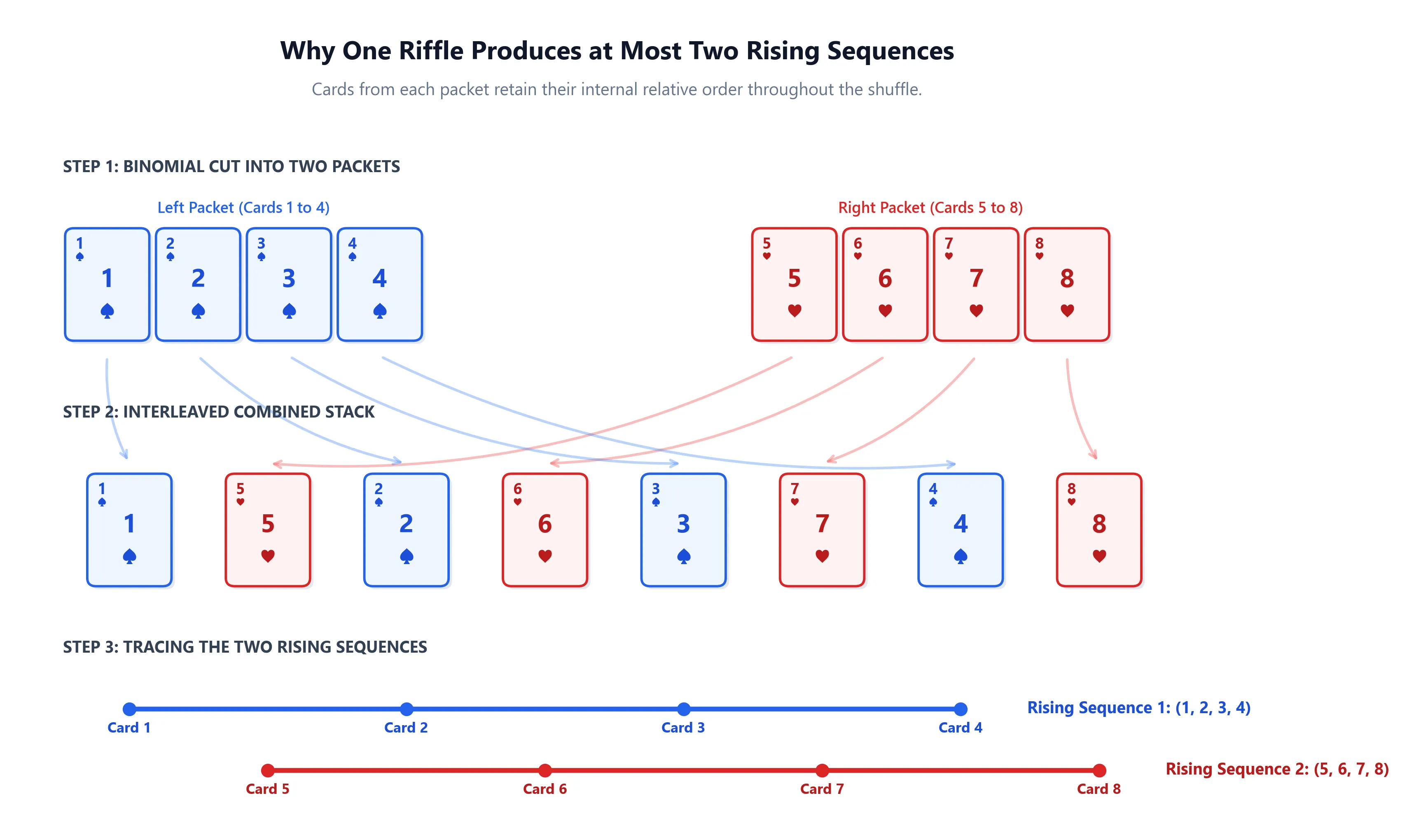
The reason is elementary: a single riffle shuffle cuts the deck into two ordered packets. When those packets drop onto the table, the relative order of cards within each packet is preserved. The cards from the left packet form one rising sequence, and the cards from the right packet form the second rising sequence. (In the degenerate case where one packet is empty, there is only 1 rising sequence.)

What happens when you shuffle the deck a second time?

Each existing rising sequence can at most be cut in two by the new cut point and interleaved. Therefore:

Theorem (Sequence Doubling):
After $k$ independent GSR riffle shuffles, the resulting permutation can have at most $2^k$ rising sequences.

Let us evaluate this bound for a standard 52-card deck:

• After $1$ shuffle: at most $2^1 = 2$ rising sequences.
• After $2$ shuffles: at most $2^2 = 4$ rising sequences.
• After $3$ shuffles: at most $2^3 = 8$ rising sequences.
• After $4$ shuffles: at most $2^4 = 16$ rising sequences.
• After $5$ shuffles: at most $2^5 = 32$ rising sequences.

Now pause and consider what a truly random permutation of 52 cards looks like.

3. Eulerian Numbers and the Reachability Barrier

In an average, randomly chosen permutation of $n$ cards, how many rising sequences would you expect to find?

The answer comes from classical combinatorics. The number of permutations in the symmetric group $S_n$ that have exactly $r$ rising sequences is given by the Eulerian numbers, denoted $A(n, r)$ (or $\left\langle \begin{matrix} n \\ r-1 \end{matrix} \right\rangle$):

$A(n, r) = \sum_{j=0}^{r} (-1)^j \binom{n+1}{j} (r - j)^n$

Eulerian numbers are symmetric: $A(n, r) = A(n, n - r + 1)$. The distribution is bell-shaped and centered at:

$\mathbb{E}[R] = \frac{n + 1}{2}$

For a 52-card deck:

$\mathbb{E}[R] = \frac{52 + 1}{2} = 26.5$

A genuinely random permutation of 52 cards typically has between 23 and 30 rising sequences. Permutations with fewer than 17 rising sequences are astronomically rare:

$\sum_{r=1}^{16} A(52, r) \approx 1.83 \times 10^{65}$

While $1.83 \times 10^{65}$ sounds like a large number, recall that $52! \approx 8.0658 \times 10^{67}$. The fraction of all permutations having 16 or fewer rising sequences is:

$\frac{\sum_{r=1}^{16} A(52, r)}{52!} \approx 0.00226 \quad (0.226\%)$

This reveals the reachability barrier:

• After 4 shuffles, the maximum number of rising sequences a deck can possibly have is $2^4 = 16$.
• Therefore, after 4 shuffles, over 99.77% of all possible permutations have probability strictly zero.

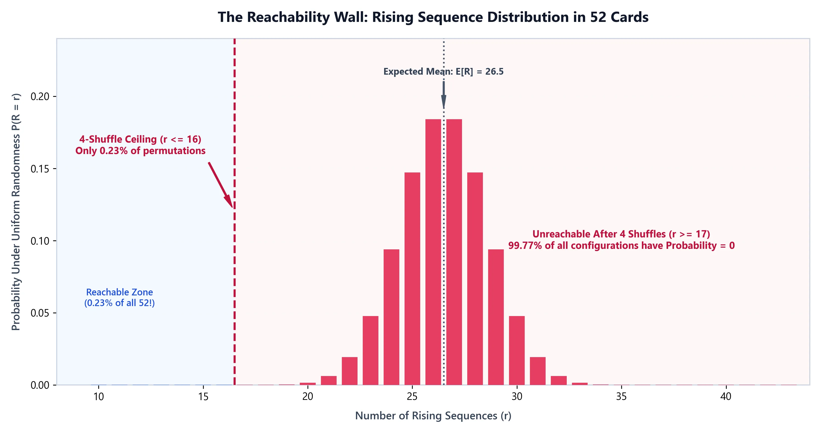
You cannot reach them. No matter which cards fall where, 4 shuffles physically cannot generate any permutation that requires 17 or more rising sequences. The dealer has not shuffled the deck into a random state; they have confined it to a microscopic subset comprising less than a quarter of one percent of the permutation group.

Even after 5 shuffles, where $2^5 = 32$, any permutation requiring 33 or more rising sequences has probability exactly zero.

4. The Bayer-Diaconis Probability Formula

In their 1992 paper, Bayer and Diaconis went far beyond counting reachability. They derived the exact probability distribution over the entire symmetric group $S_n$ after $k$ shuffles.

Their insight relied on an equivalence between shuffling and reading expansion digits. Consider marking each card with an independent uniform random binary digit in $\{0, 1\}$. Sorting the deck stably by this bit (keeping cards with 0 in their initial relative order, followed by cards with 1 in their initial relative order) is precisely a GSR shuffle.

Performing $k$ successive shuffles corresponds to assigning each card a random $k$-bit binary label:

$b_i = (b_{i, 1}, b_{i, 2}, \dots, b_{i, k}) \in \{0, 1\}^k$

and sorting the cards lexicographically by their $k$-bit labels, breaking ties using their initial positions. Since there are $a = 2^k$ possible values for a $k$-bit label, $k$ shuffles are equivalent to a single $a$-shuffle, where the deck is cut into $a$ packets according to a multinomial distribution and then interleaved.

Using this geometric and algebraic formulation, Bayer and Diaconis proved:

Theorem (Bayer & Diaconis, 1992):
Let $\sigma \in S_n$ be a permutation with $r = R(\sigma)$ rising sequences. The exact probability of arriving at $\sigma$ after $k$ independent GSR riffle shuffles is:

$Q^k(\sigma) = \frac{\binom{2^k + n - r}{n}}{2^{k n}}$

This is an astonishingly clean formula. The probability of obtaining a permutation $\sigma$ does not depend on the individual values of its cards or their complex pairings. It depends solely on a single integer: the number of rising sequences $r$ in $\sigma$.

Let us examine what this formula tells us:

• If $r > 2^k$, then $2^k + n - r < n$, and the binomial coefficient $\binom{2^k + n - r}{n} = 0$. The probability is zero, matching our earlier combinatorial bound.
• When $k$ becomes large, $2^k \gg n$, and the binomial coefficient can be approximated using Stirling’s expansion: $\binom{2^k + n - r}{n} \approx \frac{(2^k)^n}{n!}$ Then $Q^k(\sigma) \to \frac{1}{n!}$, which is the uniform distribution.

5. Total Variation Distance and the Cutoff

To quantify how close the distribution $Q^k$ is to the uniform distribution $U(\sigma) = 1/n!$, probabilists use the total variation distance ($d_{\text{TV}}$):

$\|Q^k - U\|_{\text{TV}} = \max_{A \subseteq S_n} |Q^k(A) - U(A)| = \frac{1}{2} \sum_{\sigma \in S_n} \left| Q^k(\sigma) - \frac{1}{n!} \right|$

Total variation distance has a concrete operational meaning: it represents the maximum advantage any gambler can achieve on any event $A$ over random guessing.

• If $\|Q^k - U\|_{\text{TV}} = 1.0$, there exists an event that occurs with probability 1 under $Q^k$ but with probability near 0 under $U$. The deck is completely non-random.
• If $\|Q^k - U\|_{\text{TV}} = 0.0$, the distribution is indistinguishable from uniform randomness.

Because $Q^k(\sigma)$ is identical for all permutations with the same number of rising sequences $r$, and because there are exactly $A(n, r)$ such permutations, the sum over all $52!$ configurations collapses to a simple 52-term sum:

$\|Q^k - U\|_{\text{TV}} = \frac{1}{2} \sum_{r=1}^{n} A(n, r) \left| \frac{\binom{2^k + n - r}{n}}{2^{k n}} - \frac{1}{n!} \right|$

Evaluating this sum for $n = 52$ yields the exact numbers:

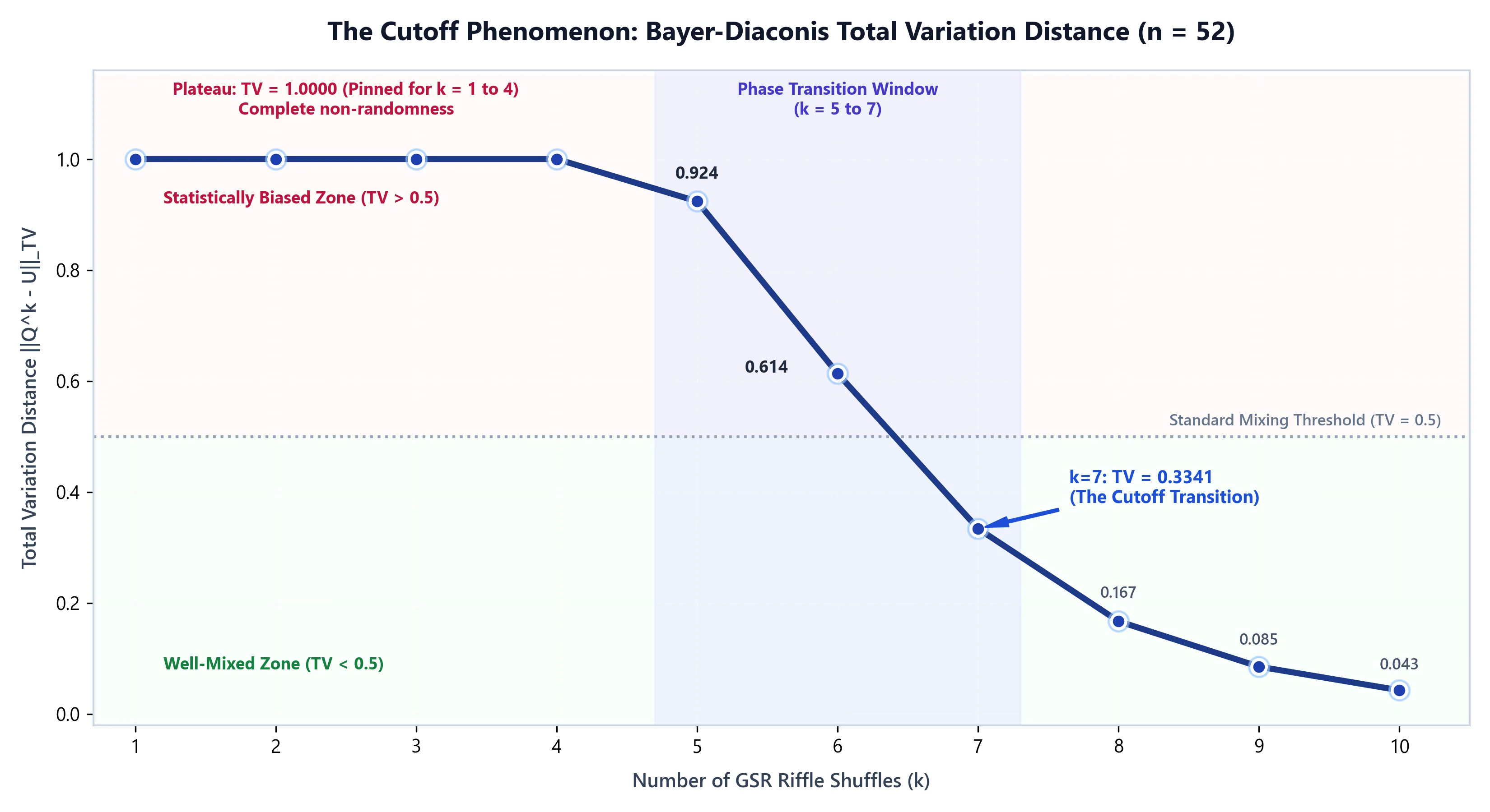
For the first four shuffles, the variation distance is effectively pinned at 1.0. The deck is not mixing gradually.

Then, between shuffles 5 and 7, the distance plunges precipitously: from $0.924$ down to $0.334$. After shuffle 7, each subsequent shuffle cuts the remaining variation distance roughly in half: $0.167$ at 8, $0.085$ at 9, and $0.043$ at 10.

This step-function behavior is known as the cutoff phenomenon. Rather than decaying exponentially from time zero like a standard diffusive physical system, the Markov chain stays far from equilibrium for a fixed duration, and then rapidly transitions to its stationary distribution within a narrow window.

6. The Asymptotic Scaling Law

Why does the cutoff occur at 7 for a 52-card deck? What happens if you shuffle a deck of 100 cards, or 1,000 cards?

Bayer and Diaconis proved that as $n \to \infty$, the critical number of shuffles scales logarithmically with the deck size:

$k(n) = \frac{3}{2} \log_2(n) + \theta$

where $\theta$ is a constant offset parameterizing the position inside the transition window.

Specifically, if you set $k = \frac{3}{2} \log_2(n) + c$, then as $n \to \infty$:

$\|Q^k - U\|_{\text{TV}} \to 1 - 2 \Phi\left( -\frac{2^{-c}}{4 \sqrt{3}} \right)$

where $\Phi(x) = \frac{1}{\sqrt{2\pi}} \int_{-\infty}^x e^{-t^2/2} dt$ is the standard normal cumulative distribution function.

Let us check the leading term for a standard deck:

$\frac{3}{2} \log_2(52) = 1.5 \times 5.7004 \approx 8.55$

Finite-size combinatorial corrections shift the inflection point slightly to the left, centering the drop between $k = 5$ and $k = 7$.

Contrast this scaling with other types of physical shuffles:

1. Top-to-Random Shuffle: Take the top card and insert it at a uniform random position in the deck. The mixing time is $O(n \log n)$. For 52 cards, this requires roughly $52 \ln(52) \approx 205$ moves.
2. Random Transpositions: Pick two cards uniformly at random and swap them. The mixing time is $O(n \log n)$, requiring roughly 100 swaps.
3. Overhand Shuffle: The casual shuffling method where small packets are slipped from one hand to the other. Its mixing time is $O(n^2 \log n)$. To randomize a 52-card deck using overhand shuffles alone, you need approximately 2,500 shuffles.

Because the riffle shuffle operates on all $n$ cards simultaneously through binary interleaving, it requires only $O(\log n)$ operations, making it one of the most efficient physical mixing algorithms known.

7. Python Implementation: Verifying the Exact Numbers

You do not have to take the theorem on faith. The exact total variation distances can be computed directly using Python’s standard library:

1
import math
2

3
def eulerian_number(n: int, r: int) -> int:
4
    """
5
    Computes the Eulerian number A(n, r): the number of permutations
6
    in S_n having exactly r rising sequences.
7
    """
8
    return sum(
9
        (-1)**j * math.comb(n + 1, j) * ((r - j)**n)
10
        for j in range(r + 1)
11
    )
12

13
def bayer_diaconis_tv(n: int, max_k: int = 10) -> list[tuple[int, float]]:
14
    """
15
    Computes exact total variation distance for a deck of size n
16
    after k = 1 ... max_k Gilbert-Shannon-Reeds riffle shuffles.
17
    """
18
    n_factorial = math.factorial(n)
19

20
    # Precompute Eulerian numbers A(n, 1) through A(n, n)
21
    eulerian = [eulerian_number(n, r) for r in range(1, n + 1)]
22
    assert sum(eulerian) == n_factorial, "Eulerian sum must equal n!"
23

24
    results = []
25
    for k in range(1, max_k + 1):
26
        two_k = 2**k
27
        two_kn = 2**(k * n)
28

29
        tv_numerator = 0
30
        for r in range(1, n + 1):
31
            count = eulerian[r - 1]
32
            # Q^k(sigma) = comb(2^k + n - r, n) / 2^(k*n)
33
            # Uniform U(sigma) = 1 / n!
34
            # We scale both terms by n! * 2^(kn) to work with exact integers:
35
            prob_scaled = math.comb(two_k + n - r, n) * n_factorial
36
            unif_scaled = two_kn
37
            tv_numerator += count * abs(prob_scaled - unif_scaled)
38

39
        # Divide by 2 * n! * 2^(kn)
40
        tv_distance = tv_numerator / (2 * n_factorial * two_kn)
41
        results.append((k, tv_distance))
42

43
    return results
44

45
if __name__ == "__main__":
46
    n = 52
47
    print(f"Bayer-Diaconis Total Variation Distance for n = {n}:")
48
    print(f"{'k':>3} | {'TV Distance':>12}")
49
    print("-" * 18)
50
    for k, tv in bayer_diaconis_tv(n, max_k=10):
51
        print(f"{k:3d} | {tv:12.4f}")

Running this script takes less than one second and outputs the exact values derived by Bayer and Diaconis in 1992:

Bayer-Diaconis Total Variation Distance for n = 52:
  k |  TV Distance
------------------
  1 |       1.0000
  2 |       1.0000
  3 |       1.0000
  4 |       1.0000
  5 |       0.9237
  6 |       0.6135
  7 |       0.3341
  8 |       0.1672
  9 |       0.0854
 10 |       0.0429

8. Exploiting the Defect: A Simple Practical Test

Why does a total variation distance of $1.0000$ matter to a player at a table?

Suppose you are playing a game where a dealer shuffles a new deck 3 times and begins dealing cards one by one from the top. Can you exploit the order?

Yes, easily. Consider this simple prediction rule:

Guess: Whenever a card is dealt, guess that the next card will have a higher value if the current card belongs to an unfinished rising sequence.

Because 3 shuffles can produce at most $2^3 = 8$ rising sequences, the cards in the deck are partitioned into at most 8 long monotonic threads. On average, each thread contains $52 / 8 = 6.5$ cards.

Under genuine randomness, the chance that the next card is higher than the current card is roughly $50\%$. But after only 3 or 4 shuffles:

• If the card just dealt is a 4, there is a very high probability that the 5 from that same original packet is sitting just a few cards deeper in the stack.
• The probability of correctly guessing whether the next card is higher or lower rises from $50\%$ to over $75\%$.

Persi Diaconis once demonstrated this to casino executives. He bet that after 4 shuffles, he could consistently predict whether upcoming cards were red or black, high or low, with statistical significance. When they saw the results, several major casino operators changed their dealer procedures, requiring automated shuffling machines or mandating at least seven riffle shuffles combined with a box cut before dealing.

9. Conclusion

Most people stop after three or four riffle shuffles because the cards already look thoroughly mixed. Every card has moved, neighboring pairs have been split up, and red and black cards alternate across the spread. But local disorder is deceptive.

A riffle shuffle only doubles the number of rising sequences each time it is performed. Because a typical 52-card permutation requires around 26 rising sequences, four shuffles leave more than 99% of all possible configurations completely out of reach. The variation distance does not decay gradually from the start; it stays pinned near 1.0 until a sharp cutoff between the fifth and seventh shuffle. It takes seven riffles to actually wash out that structural memory. Anything less, and the deck still retains a clear imprint of where it began.