spectral graphs are fun :D

Two common problems in graph theory look purely combinatorial on the surface:

1. Graph Layout: Given a set of vertices and edges, compute coordinates $(x_u, y_u)$ for each vertex in 2D space such that connected vertices are positioned near each other while avoiding unnecessary edge crossings.
2. Graph Partitioning: Partition the vertices into two subsets of roughly equal size such that the number of cut edges across the partition is minimized.

Finding the optimal balanced partition (minimizing conductance) is NP hard. Yet both problems can be approximated directly using linear algebra by computing the eigenvectors of a single symmetric matrix called the Graph Laplacian.

1. The Graph Laplacian and Quadratic Forms

Let $G = (V, E)$ be an undirected, unweighted graph with $n$ vertices.

We define two matrices associated with $G$:

• The Degree Matrix ($D$): an $n \times n$ diagonal matrix where $D_{uu} = \text{deg}(u)$ is the degree of vertex $u$.
• The Adjacency Matrix ($A$): an $n \times n$ symmetric matrix where $A_{uv} = 1$ if $(u, v) \in E$, and $A_{uv} = 0$ otherwise.

The Graph Laplacian $L$ is defined as:

$L = D - A$

Suppose we assign a real value $x_u \in \mathbb{R}$ to each vertex $u$, forming a vector $x = (x_1, \dots, x_n)^T \in \mathbb{R}^n$. Evaluating the quadratic form $x^T L x$ gives:

$x^T L x = x^T D x - x^T A x = \sum_{u \in V} \text{deg}(u) x_u^2 - 2 \sum_{(u, v) \in E} x_u x_v$

Since $\text{deg}(u) = \sum_{v : (u, v) \in E} 1$, we can rewrite the first sum over edges:

$x^T L x = \sum_{(u, v) \in E} (x_u - x_v)^2$

This formulation reveals the physical intuition behind $L$. If we view each edge as a unit spring connecting vertices along a 1D coordinate axis, $x^T L x$ represents the total potential energy of the system. Minimizing $x^T L x$ corresponds to finding vertex positions that minimize the total squared distance between connected pairs.

Because $(x_u - x_v)^2 \ge 0$ for every edge, $x^T L x \ge 0$ for all $x \in \mathbb{R}^n$. Thus, $L$ is positive semidefinite ($L \succeq 0$), and all its eigenvalues are real and nonnegative:

$0 = \lambda_1 \le \lambda_2 \le \lambda_3 \le \dots \le \lambda_n$

2. The Trivial Solution and the Fiedler Vector

If we simply minimize $x^T L x$ without constraints, the minimum is 0, achieved by setting all $x_u$ equal to a constant $c$.

This corresponds to the all ones vector $\mathbf{1} = (1, 1, \dots, 1)^T$:

$L \mathbf{1} = (D - A)\mathbf{1} = \mathbf{0}$

Thus, $\lambda_1 = 0$ is always an eigenvalue of $L$ with eigenvector $v_1 = \mathbf{1}$. In general, the multiplicity of the 0 eigenvalue equals the number of connected components in $G$.

To obtain a nontrivial coordinate assignment, we enforce two normalization conditions:

1. Centering at the origin: $\sum_{u \in V} x_u = 0$, which is equivalent to $x \perp \mathbf{1}$.
2. Fixed variance: $\sum_{u \in V} x_u^2 = 1$, which is equivalent to $\|x\|_2 = 1$.

We then consider the constrained optimization problem:

$\min_{\substack{\|x\|_2 = 1 \\ x \perp \mathbf{1}}} x^T L x$

By the Rayleigh Ritz theorem, the solution to this problem is given by the eigenvector corresponding to the second smallest eigenvalue $\lambda_2$ of $L$.

This eigenvector $v_2$ is known as the Fiedler vector, and $\lambda_2$ is called the algebraic connectivity of the graph.

3. A Worked Example: The Four Node Path Graph

Consider a four node path graph:

1
(1) === (2) === (3) === (4)

The degree matrix $D$ and adjacency matrix $A$ are:

$D = \begin{pmatrix} 1 & 0 & 0 & 0 \\ 0 & 2 & 0 & 0 \\ 0 & 0 & 2 & 0 \\ 0 & 0 & 0 & 1 \end{pmatrix}, \quad A = \begin{pmatrix} 0 & 1 & 0 & 0 \\ 1 & 0 & 1 & 0 \\ 0 & 1 & 0 & 1 \\ 0 & 0 & 1 & 0 \end{pmatrix}$

The Laplacian $L = D - A$ is:

$L = \begin{pmatrix} 1 & -1 & 0 & 0 \\ -1 & 2 & -1 & 0 \\ 0 & -1 & 2 & -1 \\ 0 & 0 & -1 & 1 \end{pmatrix}$

The characteristic polynomial of $L$ factors as:

$\det(L - \lambda I) = \lambda (\lambda - 2) (\lambda^2 - 4\lambda + 2) = 0$

The eigenvalues are:

$\lambda_1 = 0, \quad \lambda_2 = 2 - \sqrt{2} \approx 0.586, \quad \lambda_3 = 2.0, \quad \lambda_4 = 2 + \sqrt{2} \approx 3.414$

The normalized Fiedler eigenvector $v_2$ for $\lambda_2 = 2 - \sqrt{2}$ is:

$v_2 = \frac{1}{2} \begin{pmatrix} -\sqrt{1 + 1/\sqrt{2}} \\ -\sqrt{1 - 1/\sqrt{2}} \\ +\sqrt{1 - 1/\sqrt{2}} \\ +\sqrt{1 + 1/\sqrt{2}} \end{pmatrix} \approx \begin{pmatrix} -0.653 \\ -0.271 \\ +0.271 \\ +0.653 \end{pmatrix}$

The entries of $v_2$ assign coordinates to the vertices in order along a 1D line:

• $v_2(1) \approx -0.653$
• $v_2(2) \approx -0.271$
• $v_2(3) \approx +0.271$
• $v_2(4) \approx +0.653$

The eigenvector recovers the linear ordering and symmetric spacing of the path graph purely from the entries of $L$.

4. 2D Spectral Graph Drawing

To embed a graph in $\mathbb{R}^2$, we compute two orthogonal 1D coordinate assignments.

We choose:

• x coordinates from the second eigenvector: $x = v_2$
• y coordinates from the third eigenvector: $y = v_3$ (which satisfies $v_3 \perp \mathbf{1}$ and $v_3 \perp v_2$)

Each vertex $u$ is plotted at the point $(v_2(u), v_3(u))$.

The figure below compares embeddings generated by the smallest nontrivial eigenvectors $(v_2, v_3)$ against embeddings generated by the largest eigenvectors $(v_n, v_{n-1})$:

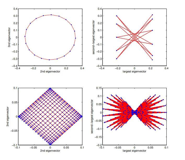
Mathematical Basis for the Layouts:

• Top Left (20 node cycle with $v_2, v_3$): The Laplacian of a cycle graph is a circulant matrix. Its eigenvectors are discrete Fourier modes of the form $v(k) = (\cos(2\pi j k / n))_{j=1}^n$ and $(\sin(2\pi j k / n))_{j=1}^n$. Plotting $(v_2, v_3)$ evaluates the fundamental frequency ($k=1$), reconstructing a regular polygon in the plane.
• Top Right (20 node cycle with $v_n, v_{n-1}$): The largest eigenvectors maximize the quadratic form $\sum (x_u - x_v)^2$, forcing adjacent vertices to opposite sides of the origin.
• Bottom Left ($20 \times 20$ grid with $v_2, v_3$): The Cartesian product structure of the grid yields tensor product eigenvectors that untangle the vertices into a planar grid.
• Bottom Right ($20 \times 20$ grid with $v_n, v_{n-1}$): High frequency eigenmodes create a heavily self intersecting configuration.

5. Spectral Graph Partitioning

The Fiedler vector also provides an approximation for the graph cut problem.

For a subset of vertices $S \subset V$, let $\bar{S} = V \setminus S$. The conductance $\phi(S)$ is defined as:

$\phi(S) = \frac{|E(S, \bar{S})|}{\min(|S|, |\bar{S}|)}$

Where $|E(S, \bar{S})|$ is the number of edges with one endpoint in $S$ and one in $\bar{S}$. The conductance of the graph is:

$\phi(G) = \min_{\substack{S \subset V \\ 0 < |S| \le |V|/2}} \phi(S)$

Finding the subset $S$ that minimizes conductance is NP hard. The Sweep Cut algorithm uses $v_2$ to find an approximate solution:

1. Compute the Fiedler vector $v_2$ of $L$.
2. Sort the vertices such that $v_2(u_1) \le v_2(u_2) \le \dots \le v_2(u_n)$.
3. Evaluate the conductance of each prefix set $S_k = \{u_1, \dots, u_k\}$ for $k = 1, \dots, n-1$.
4. Select the prefix cut that achieves the minimum conductance.

In our four node path example, $v_2 = (-0.653, -0.271, +0.271, +0.653)$. The sign changes between vertices 2 and 3. The partition $S = \{1, 2\}$ and $\bar{S} = \{3, 4\}$ cuts exactly 1 edge with $|S| = 2$, yielding conductance $\phi(S) = 1/2$, which is optimal.

Cheeger’s Inequality

The theoretical guarantee for spectral partitioning is provided by Cheeger’s Inequality (adapted to graphs by Alon and Milman):

$\frac{\lambda_2}{2} \le \phi(G) \le \sqrt{2 d_{\max} \lambda_2}$

Where $d_{\max}$ is the maximum degree in $G$.

This inequality establishes that:

• If $\lambda_2$ is close to 0, there exists a cut with small conductance (a sparse bottleneck).
• If $\lambda_2$ is bounded away from 0, the graph is an expander graph, and no sparse cut exists.

6. Implementation

The following Python function computes the 2D spectral coordinates and performs the sweep cut on a sparse adjacency matrix:

1
import numpy as np
2
import scipy.sparse as sp
3
import scipy.sparse.linalg as sla
4

5
def spectral_embedding(adj_matrix):
6
    """Computes 2D coordinates (v2, v3) from the Graph Laplacian."""
7
    degrees = np.array(adj_matrix.sum(axis=1)).flatten()
8
    n = len(degrees)
9

10
    # Construct Laplacian L = D - A
11
    L = sp.diags(degrees) - adj_matrix
12

13
    # Compute the 3 smallest eigenvalues and eigenvectors
14
    vals, vecs = sla.eigsh(L.astype(float), k=3, which='SM')
15

16
    order = np.argsort(vals)
17
    v2 = vecs[:, order[1]]
18
    v3 = vecs[:, order[2]]
19

20
    return v2, v3
21

22
def sweep_cut(adj_matrix):
23
    """Finds the minimal conductance cut along the Fiedler vector."""
24
    v2, _ = spectral_embedding(adj_matrix)
25
    order = np.argsort(v2)
26
    n = len(order)
27

28
    best_cond = float('inf')
29
    best_split = None
30

31
    for k in range(1, n):
32
        S = set(order[:k])
33
        cut_edges = sum(
34
            1 for u in S
35
            for v in adj_matrix[u].indices
36
            if v not in S
37
        )
38
        cond = cut_edges / min(len(S), n - len(S))
39

40
        if cond < best_cond:
41
            best_cond = cond
42
            best_split = S
43

44
    return best_split, best_cond

7. Summary